python链表冒泡排序、二叉树顺序递归遍历、顺序表的快排
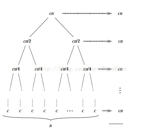
一、python实现链表冒泡排序 - 冒泡排序的概念:冒泡排序是一种交换排序,它的基本思想是:两两比较相邻记录的关键字,如果反序则交换,直至没有反序的记录为止。因为按照该算法,每次比较会将当前未排序的记录序列中最小的关键字移至未排序的记录序列最前(或者将当前未排序的记录序列中最大的关键字移至未排序的记录序列最后),就像冒泡一样,故以此为名。 - 冒泡排序算法的算法描述如下: -- 比较相邻的元素。如果第一个比第二个大,就交换他们两个。 -- 对每一对相邻元素作同样的工作,从开始第一对到结尾的最后一对。这步做完后,最后的元素会是最大的数。 -- 针对所有的元素重复以上的步骤,除了最后一个。 -- 持续每次对越来越少的元素重复上面的步骤,直到没有任何一对数字需要比较。 1、基本的冒泡排序实现: li = [23, 43, 1, 2, 4, 5, 253] def bubble(li): if not len(li): return count = 0 for i in range(len(li)): for j in range(len(li) - 1): count+=1 if li[i] < li[j]: li[i], li[j] = li[j], li[i] print(count) return li ret_li = bubble(li) print(ret_li) 42 //循环的次数 [1, 2, 4, 5, 23, 43, 253] //排序结果 2、基本优化 这种方法利用了双重循环,会造成不必要的比较,所以优化一下,可以考虑从尾部开始,这样可以将以排好序的部分不再检查 def bubble(li): if not len(li): return count = 0 for i in range(len(li)): j = len(li) - 1 while j > i: count +=1 if li[j] < li[j - 1]: li[j], li[j - 1] = li[j - 1], li[j] j -= 1 print(count) return li ret_li = bubble(li) print(ret_li) 21//循环的次数 [1, 2, 4, 5, 23, 43, 253] //排序结果 3、进一步优化 通过设置flag来判断某次循环是否没有出现位置交换,没有交换就说明排序已完成 def bubble(li): if not len(li): return count = 0 for i in range(len(li)): flag = False j = len(li) - 1 while j > i: count += 1 if li[j] < li[j - 1]: li[j], li[j - 1] = li[j - 1], li[j] flag = True j -= 1 if not flag: print(count) return li return li ret_li = bubble(li) print(ret_li) 20 //循环次数 [1, 2, 4, 5, 23, 43, 253] //排序结果 二、二叉树的顺序遍历 二叉树是有限个元素的集合,该集合或者为空、或者有一个称为根节点(root)的元素及两个互不相交的、分别被称为左子树和右子树的二叉树组成。 -- 二叉树的每个结点至多只有二棵子树(不存在度大于2的结点),二叉树的子树有左右之分,次序不能颠倒。 -- 二叉树的第i层至多有2^{i-1}个结点 -- 深度为k的二叉树至多有2^k-1个结点; -- 对任何一棵二叉树T,如果其终端结点数为N0,度为2的结点数为N2,则N0=N2+1 二叉树有三种遍历方式:先序遍历,中序遍历,后续遍历 即:先中后指的是访问根节点的顺序 eg:先序 根左右 中序 左根右 后序 左右根 遍历总体思路:将树分成最小的子树,然后按照顺序输出 #实现树结构的类,树的节点有三个私有属性 左指针 右指针 自己的值 class Node(): def __init__(self,data =None,left=None,right = None): self._data = data self._left = left self._right = right #先序遍历 遍历过程 根左右 def pro_order(tree): if tree == None: return False print(tree._data) pro_order(tree._left) pro_order(tree._right) #后序遍历 遍历过程 左右根 def pos_order(tree): if tree == None: return False # print(tree.get_data()) pos_order(tree._left) pos_order(tree._right) print(tree._data) #中序遍历 遍历过程 左根右 def mid_order(tree): if tree == None: return False # print(tree.get_data()) mid_order(tree._left) print(tree._data) mid_order(tree._right) #层次遍历 def row_order(tree): # print(tree._data) queue = [] queue.append(tree) while True: if queue==[]: break print(queue[0]._data) first_tree = queue[0] if first_tree._left != None: queue.append(first_tree._left) if first_tree._right != None: queue.append(first_tree._right) queue.remove(first_tree) if __name__ == '__main__': tree = Node('A',Node('B',Node('D'),Node('E')),Node('C',Node('F'),Node('G'))) pro_order(tree) mid_order(tree) pos_order(tree) row_order(tree) 三、python实现顺序表的快排 1、快排的介绍: 快速排序采用的思想是分治思想,先简单的介绍一下分治的思想。分治算法的基本思想是将一个规模为N的问题分解为K个规模较小的子问题,这些子问题相互独立且与原问题性质相同。求出子问题的解,就可以得到原问题的解。下面这张图会说明分治算法是如何进行的:将cn分成了两个cn/2,转而分成了cn/4,cn/8......我们通过这样一层一层的求解规模小的子问题,将其合并之后就能求出原问题的解。 图解.jpg 2、快排的基本思路是: 在待排序的序列中选取一个值作为一个基准值,按照这个基准值得大小将这个序列划分成两个子序列,基准值会在这两个子序列的中间,一边是比基准小的,另一边就是比基准大的。这样快速排序第一次排完,我们选取的这个基准值就会出现在它该出现的位置上。这就是快速排序的单趟算法,也就是完成了一次快速排序。然后再对这两个子序列按照同样的方法进行排序,直到只剩下一个元素或者没有元素的时候就停止,这时候所有的元素都出现在了该出现的位置上。 附图:快排的图解 快排.jpg 3、快排的特点 快速排序之所比较快,因为相比冒泡排序,每次交换是跳跃式的。每次排序的时候设置一个基准点,将小于等于基准点的数全部放到基准点的左边,将大于等于基准点的数全部放到基准点的右边。这样在每次交换的时候就不会像冒泡排序一样每次只能在相邻的数之间进行交换,交换的距离就大的多了。因此总的比较和交换次数就少了,速度自然就提高了。当然在最坏的情况下,仍可能是相邻的两个数进行了交换。因此快速排序的最差时间复杂度和冒泡排序是一样的都是O(N2),它的平均时间复杂度为O(NlogN)。其实快速排序是基于一种叫做“二分”的思想。 4、快排的代码实现 def quick_sort(li): if len(li) <= 1: return li base_value = li[len(li) // 2] left_part = [item for item in li if item < base_value] right_part = [item for item in li if item > base_value] eq_part = [item for item in li if item == base_value] return quick_sort(left_part) + eq_part + quick_sort(right_part) print(quick_sort(li = [23, 43, 1, 2, 4, 5, 253])) 简洁版的快排,两种代码其实是一样的 def quick_sort(li): if len(li) <= 1: return li return quick_sort([item for item in li[1:] if item < li[0]])+ li[0:1] + quick_sort([item for item in li[1:] if item > li[0]]) print(quick_sort(li = [23, 43, 1, 2, 4, 5, 253]))