Python3数据分析——（1）NumPy快速入门教程（官网教程翻译）

先决条件

在阅读这个教程之前，你多少需要知道点Python。如果你想从新回忆下，请看看Python Tutorial.

在阅读本教程之前，您应该了解一些Python。如果你想刷新你的记忆，请看看Python教程

基础篇

例如，在3D空间一个点的坐标[1, 2, 3]是一个秩为1的数组，因为它只有一个轴。那个轴长度为3.又例如，在以下例子中，数组的秩为2(它有两个维度).第一个维度长度为2,第二个维度长度为3.

[[ 1., 0., 0.], [ 0., 1., 2.]]

NumPy的数组类被称作ndarray。通常被称作数组。注意numpy.array和标准Python库类array.array并不相同，后者只处理一维数组和提供少量功能。更多重要ndarray对象属性有：

• ndarray.ndim

  数组轴的个数，在python的世界中，轴的个数被称作秩

• ndarray.shape

  数组的维度。这是一个指示数组在每个维度上大小的整数元组。例如一个n排m列的矩阵，它的shape属性将是(2,3),这个元组的长度显然是秩，即维度或者ndim属性

• ndarray.size

  数组元素的总个数，等于shape属性中元组元素的乘积。

• ndarray.dtype

  一个用来描述数组中元素类型的对象，可以通过创造或指定dtype使用标准Python类型。另外NumPy提供它自己的数据类型。

• ndarray.itemsize

  数组中每个元素的字节大小。例如，一个元素类型为float64的数组itemsiz属性值为8(=64/8),又如，一个元素类型为complex32的数组itemsize属性为4(=32/8).

• ndarray.data

  包含实际数组元素的缓冲区，通常我们不需要使用这个属性，因为我们总是通过索引来使用数组中的元素。

一个例子

>>> import numpy as np >>> a = np.arange(15).reshape(3, 5) >>> a array([[ 0, 1, 2, 3, 4],  [ 5, 6, 7, 8, 9],  [10, 11, 12, 13, 14]]) >>> a.shape (3, 5) >>> a.ndim 2 >>> a.dtype.name 'int64' >>> a.itemsize 8 >>> a.size 15 >>> type(a) <type 'numpy.ndarray'> >>> b = np.array([6, 7, 8]) >>> b array([6, 7, 8]) >>> type(b) <type 'numpy.ndarray'>

创建数组

有好几种创建数组的方法。

例如，你可以使用array函数从常规的Python列表和元组创造数组。所创建的数组类型由原序列中的元素类型推导而来。

>>> import numpy as np >>> a = np.array( [2,3,4] ) >>> a array([2, 3, 4]) >>> a.dtypedtype('int32') >>> b = np.array([1.2, 3.5, 5.1]) >>> b.dtype dtype('float64') 一个常见的错误包括用多个数值参数调用`array`而不是提供一个由数值组成的列表作为一个参数。 >>> a = np.array(1,2,3,4) # WRONG >>> a = np.array([1,2,3,4]) # RIGHT

数组将序列包含序列转化成二维的数组，序列包含序列包含序列转化成三维数组等等。

>>> b = np.array( [ (1.5,2,3), (4,5,6) ] ) >>> b array([[ 1.5, 2. , 3. ], [ 4. , 5. , 6. ]])

数组类型可以在创建时显示指定

>>> c = np.array( [ [1,2], [3,4] ], np.dtype=complex ) >>> c array([[ 1.+0.j, 2.+0.j], [ 3.+0.j, 4.+0.j]])

通常，数组的元素开始都是未知的，但是它的大小已知。因此，NumPy提供了一些使用占位符创建数组的函数。这最小化了扩展数组的需要和高昂的运算代价。

函数zeros创建一个全是0的数组，函数ones创建一个全1的数组，函数empty创建一个内容随机并且依赖与内存状态的数组。默认创建的数组类型(dtype)都是float64。

>>> np.zeros( (3,4) ) array([[0., 0., 0., 0.], [0., 0., 0., 0.], [0., 0., 0., 0.]]) >>> np.ones( (2,3,4), np.dtype=int16 ) # dtype can also be specified array([[[ 1, 1, 1, 1], [ 1, 1, 1, 1], [ 1, 1, 1, 1]], [[ 1, 1, 1, 1], [ 1, 1, 1, 1], [ 1, 1, 1, 1]]], np.dtype=int16) >>> np.empty( (2,3) ) array([[ 3.73603959e-262, 6.02658058e-154, 6.55490914e-260], [ 5.30498948e-313, 3.14673309e-307, 1.00000000e+000]])

为了创建一个数列，NumPy提供一个类似arange的函数返回数组而不是列表:

>>> np.arange( 10, 30, 5 ) array([10, 15, 20, 25]) >>> np.arange( 0, 2, 0.3 ) # it accepts float arguments array([ 0. , 0.3, 0.6, 0.9, 1.2, 1.5, 1.8])

当arange使用浮点数参数时，由于有限的浮点数精度，通常无法预测获得的元素个数。因此，最好使用函数linspace去接收我们想要的元素个数来代替用range来指定步长。

其它函数array, zeros, zeros_like, ones, ones_like, empty, empty_like, arange, linspace, rand, randn, fromfunction, fromfile参考：NumPy示例

打印数组

当你打印一个数组，NumPy以类似嵌套列表的形式显示它，但是呈以下布局：

• 最后的轴从左到右打印
• 次后的轴从顶向下打印
• 剩下的轴从顶向下打印，每个切片通过一个空行与下一个隔开

一维数组被打印成行，二维数组成矩阵，三维数组成矩阵列表。

>>> a = np.arange(6) # 1d array >>> print(a) [0 1 2 3 4 5] >>> >>> b =np.arange(12).reshape(4,3) # 2d array >>> print(b) [[ 0 1 2] [ 3 4 5] [ 6 7 8] [ 9 10 11]] >>> >>> c = np.arange(24).reshape(2,3,4) # 3d array >>> print(c) [[[ 0 1 2 3] [ 4 5 6 7] [ 8 9 10 11]] [[12 13 14 15] [16 17 18 19] [20 21 22 23]]]

查看形状操作一节获得有关reshape的更多细节

如果一个数组用来打印太大了，NumPy自动省略中间部分而只打印角落

>>> print(np.arange(10000)) [ 0 1 2 ..., 9997 9998 9999] >>> >>> print(np.arange(10000).reshape(100,100)) [[ 0 1 2 ..., 97 98 99] [ 100 101 102 ..., 197 198 199] [ 200 201 202 ..., 297 298 299] ..., [9700 9701 9702 ..., 9797 9798 9799] [9800 9801 9802 ..., 9897 9898 9899] [9900 9901 9902 ..., 9997 9998 9999]]

禁用NumPy的这种行为并强制打印整个数组，你可以设置printoptions参数来更改打印选项。

>>> set_printoptions(threshold='nan')

基本运算

数组的算术运算是按元素的。新的数组被创建并且被结果填充。

>>> a = np.array( [20,30,40,50] ) >>> b = np.arange( 4 ) >>> b array([0, 1, 2, 3]) >>> c = a-b >>> c array([20, 29, 38, 47]) >>> b**2 array([0, 1, 4, 9]) >>> 10*np.sin(a) array([ 9.12945251, -9.88031624, 7.4511316 , -2.62374854]) >>> a<35 array([True, True, False, False], dtype=bool)

不像许多矩阵语言，NumPy中的乘法运算符*指示按元素计算，矩阵乘法可以使用dot函数或创建矩阵对象实现(参见教程中的矩阵章节)

>>> A = np.array( [[1,1], ... [0,1]] ) >>> B = np.array( [[2,0], ... [3,4]] ) >>> A*B # elementwise product array([[2, 0], [0, 4]]) >>> np.dot(A,B) # matrix product >>>A.dot(B) #another matrix product array([[5, 4], [3, 4]])

有些操作符像+=和*=被用来更改已存在数组而不创建一个新的数组。

>>> a = np.ones((2,3), dtype=int) >>> b = np.random.random((2,3)) >>> a *= 3 >>> a array([[3, 3, 3], [3, 3, 3]]) >>> b += a >>> b array([[ 3.69092703, 3.8324276 , 3.0114541 ], [ 3.18679111, 3.3039349 , 3.37600289]]) >>> a += b # b is notautomatically converted to integer type  TypeError: Cannot cast ufunc add output from dtype('float64') to dtype('int64') with casting rule 'same_kind'

当运算的是不同类型的数组时，结果数组和更普遍和精确的已知(这种行为叫做upcast)。

>>> a = np.ones(3, dtype=np.int32) >>> b = np.linspace(0,pi,3) >>> b.dtype.name 'float64' >>> c = a+b >>> c array([ 1. , 2.57079633, 4.14159265]) >>> c.dtype.name 'float64' >>> d = np.exp(c*1j) >>> d array([ 0.54030231+0.84147098j, -0.84147098+0.54030231j, -0.54030231-0.84147098j]) >>> d.dtype.name 'complex128' 许多非数组运算，如计算数组所有元素之和，被作为ndarray类的方法实现 >>> a = np.random.random((2,3)) >>> a array([[ 0.6903007 , 0.39168346, 0.16524769], [ 0.48819875, 0.77188505, 0.94792155]]) >>> a.sum() 3.4552372100521485 >>> a.min() 0.16524768654743593 >>> a.max() 0.9479215542670073

这些运算默认应用到数组好像它就是一个数字组成的列表，无关数组的形状。然而，指定axis参数你可以吧运算应用到数组指定的轴上：

>>> b = np.arange(12).reshape(3,4) >>> b array([[ 0, 1, 2, 3], [ 4, 5, 6, 7], [ 8, 9, 10, 11]]) >>> >>> b.sum(axis=0) # sum of each column array([12, 15, 18, 21]) >>> >>> b.min(axis=1) # min of each row array([0, 4, 8]) >>> >>> b.cumsum(axis=1) # cumulative sum along each row array([[ 0, 1, 3, 6], [ 4, 9, 15, 22], [ 8, 17, 27, 38]])

通用函数(ufunc)

NumPy提供常见的数学函数如sin,cos和exp。在NumPy中，这些叫作“通用函数”(ufunc)。在NumPy里这些函数作用按数组的元素运算，产生一个数组作为输出。

>>> B = np.arange(3) >>> B array([0, 1, 2]) >>> np.exp(B) array([ 1. , 2.71828183, 7.3890561 ]) >>> np.sqrt(B) array([ 0. , 1. , 1.41421356]) >>> C = np.array([2., -1., 4.]) >>> np.add(B, C) array([ 2., 0., 6.])

更多函数all, alltrue, any, apply along axis, argmax, argmin, argsort, average, bincount, ceil, clip, conj, conjugate, corrcoef, cov, cross, cumprod, cumsum, diff, dot, floor, inner, inv, lexsort, max, maximum, mean, median, min, minimum, nonzero, outer, prod, re, round, sometrue, sort, std, sum, trace, transpose, var, vdot, vectorize, where 参见:NumPy示例

索引，切片和迭代

一维数组可以被索引、切片和迭代，就像列表和其它Python序列。

>>> a = np.arange(10)**3 >>> a array([ 0, 1, 8, 27, 64, 125, 216, 343, 512, 729]) >>> a[2] 8 >>> a[2:5] array([ 8, 27, 64]) >>> a[:6:2] = -1000 # equivalent to a[0:6:2] = -1000; from start to position 6, exclusive, set every 2nd element to -1000 >>> a array([-1000, 1, -1000, 27, -1000, 125, 216, 343, 512, 729]) >>> a[ : :-1] # reversed a array([ 729, 512, 343, 216, 125, -1000, 27, -1000, 1, -1000]) >>> for i in a: ... print(i**(1/3.)), ... nan 1.0 nan 3.0 nan 5.0 6.0 7.0 8.0 9.0

多维数组可以每个轴有一个索引。这些索引由一个逗号分割的元组给出。

>>> def f(x,y): ... return 10*x+y ... >>> b = np.fromfunction(f,(5,4),dtype=int) >>> b array([[ 0, 1, 2, 3], [10, 11, 12, 13], [20, 21, 22, 23], [30, 31, 32, 33], [40, 41, 42, 43]]) >>> b[2,3] 23 >>> b[0:5, 1] # each row in the second column of b array([ 1, 11, 21, 31, 41]) >>> b[ : ,1] # equivalent to the previous example array([ 1, 11, 21, 31, 41]) >>> b[1:3, : ] # each column in the second and third row of b array([[10, 11, 12, 13], [20, 21, 22, 23]])

当少于轴数的索引被提供时，确失的索引被认为是整个切片：

>>> b[-1] # the last row. Equivalent to b[-1,:] array([40, 41, 42, 43])

b[i]中括号中的表达式被当作i和一系列:，来代表剩下的轴。NumPy也允许你使用“点”像b[i,...]。

点(…)代表许多产生一个完整的索引元组必要的分号。如果x是秩为5的数组(即它有5个轴)，那么:

• x[1,2,…] 等同于 x[1,2,:,:,:],
• x[…,3] 等同于 x[:,:,:,:,3]
• x[4,…,5,:] 等同 x[4,:,:,5,:].

>>> c = np.array( [ [[ 0, 1, 2], # a 3D array (two stacked 2D arrays) ... [ 10, 12, 13]], ... [[100,101,102], ... [110,112,113]]]) >>> c.shape (2, 2, 3) >>> c[1,...] # same as c[1,:,:] or c[1] array([[100, 101, 102],  [110, 112, 113]]) >>> c[...,2] # same as c[:,:,2] array([[ 2, 13],  [102, 113]]) 

迭代多维数组是就第一个轴而言的:

>>> for row in b: ... print(row) ... [0 1 2 3] [10 11 12 13] [20 21 22 23] [30 31 32 33] [40 41 42 43]

然而，如果一个人想对每个数组中元素进行运算，我们可以使用flat属性，该属性是数组元素的一个迭代器:

>>> for element in b.flat: ... print(element), ... 0 1 2 3 10 11 12 13 20 21 22 23 30 31 32 33 40 41 42 43

更多[], …, newaxis, ndenumerate, indices, index exp 参考NumPy示例

形状操作

更改数组的形状

一个数组的形状由它每个轴上的元素个数给出：

>>> a = np.floor(10*np.random.random((3,4))) >>> a array([[ 2., 8., 0., 6.], [ 4., 5., 1., 1.], [ 8., 9., 3., 6.]]) >>> a.shape (3, 4)

一个数组的形状可以被多种命令修改：

>>> a.ravel() # returns the array,flattened 返回数组，展开 array([ 2., 8., 0., 6., 4., 5., 1., 1., 8., 9., 3., 6.]) >>> a.reshape(6, 2) #returns the array with a modified shape 返回与改变形状的阵列array([[2.,8.], [0.,6.], [4.,5.], [1.,1.], [8.,9.], [3.,6.]]) >>> a.T #returns the array,transposed 返回数组，转置 array([[ 2., 4., 8.], [ 8., 5., 9.], [ 0., 1., 3.],  [ 6., 1., 6.]])>>>a.T.shape(4,3)>>>a.shape(3,4)

由ravel()展平的数组元素的顺序通常是“C风格”的，就是说，最右边的索引变化得最快，所以元素a[0,0]之后是a[0,1]。如果数组被改变形状(reshape)成其它形状，数组仍然是“C风格”的。NumPy通常创建一个以这个顺序保存数据的数组，所以ravel()将总是不需要复制它的参数。但是如果数组是通过切片其它数组或有不同寻常的选项时，它可能需要被复制。函数reshape()和ravel()还可以被同过一些可选参数构建成FORTRAN风格的数组，即最左边的索引变化最快。

reshape函数改变参数形状并返回它，而resize函数改变数组自身。

>>> a

array([[ 2.,  8., 0.,  6.],

       [ 4., 5.,  1.,  1.],

       [8.,  9., 3.,  6.]])

>>> a.resize((2,6))

>>> a

array([[ 2.,  8., 0.,  6.],

       [ 4., 5.,  1.,  1.],

       [ 8., 9.,  3.,  6.]])

更多 shape, reshape, resize, ravel 参考NumPy示例

组合(stack)不同的数组

几种方法可以沿不同轴将数组堆叠在一起：

>>> a = floor(10*np.random.random((2,2))) >>> a array([[ 1., 1.], [ 5., 8.]]) >>> b = floor(10*random.random((2,2))) >>> b array([[ 3., 3.], [ 6., 0.]]) >>> vstack((a,b)) array([[ 1., 1.], [ 5., 8.], [ 3., 3.], [ 6., 0.]]) >>> hstack((a,b)) array([[ 1., 1., 3., 3.], [ 5., 8., 6., 0.]])

函数column_stack以列将一维数组合成二维数组，它等同与vstack对一维数组。

>>> np.column_stack((a,b)) # With 2D arrays array([[ 1., 1., 3., 3.], [ 5., 8., 6., 0.]]) >>> a=np.array([4.,2.]) >>> b=np.array([2.,8.]) >>> a[:,newaxis] # This allows to have a 2D columns vector array([[ 4.], [ 2.]]) >>> np.column_stack((a[:,newaxis],b[:,newaxis])) array([[ 4., 2.], [ 2., 8.]]) >>> np.vstack((a[:,newaxis],b[:,newaxis])) # The behavior of vstack is different array([[ 4.], [ 2.], [ 2.], [ 8.]])

row_stack函数，另一方面，将一维数组以行组合成二维数组。

对那些维度比二维更高的数组，hstack沿着第二个轴组合，vstack沿着第一个轴组合,concatenate允许可选参数给出组合时沿着的轴。

Note

在复杂情况下，r_[]和c_[]对创建沿着一个方向组合的数很有用，它们允许范围符号(“:”):

>>> np.r_[1:4,0,4] array([1, 2, 3, 0, 4])

当使用数组作为参数时，r_和c_的默认行为和vstack和hstack很像，但是允许可选的参数给出组合所沿着的轴的代号。

更多函数hstack , vstack, column_stack , row_stack , concatenate , c_ , r_ 参见NumPy示例.

将一个数组分割(split)成几个小数组

使用hsplit你能将数组沿着它的水平轴分割，或者指定返回相同形状数组的个数，或者指定在哪些列后发生分割:

>>> a = np.floor(10*np.random.random((2,12))) >>> a array([[ 8., 8., 3., 9., 0., 4., 3., 0., 0., 6., 4., 4.], [ 0., 3., 2., 9., 6., 0., 4., 5., 7., 5., 1., 4.]]) >>> np.hsplit(a,3) # Split a into 3 [array([[ 8., 8., 3., 9.], [ 0., 3., 2., 9.]]), array([[ 0., 4., 3., 0.], [ 6., 0., 4., 5.]]), array([[ 0., 6., 4., 4.], [ 7., 5., 1., 4.]])] >>> np.hsplit(a,(3,4)) # Split a after the third and the fourth column [array([[ 8., 8., 3.], [ 0., 3., 2.]]), array([[ 9.], [ 9.]]), array([[ 0., 4., 3., 0., 0., 6., 4., 4.], [ 6., 0., 4., 5., 7., 5., 1., 4.]])]

vsplit沿着纵向的轴分割，array split允许指定沿哪个轴分割。

复制和视图

当运算和处理数组时，它们的数据有时被拷贝到新的数组有时不是。这通常是新手的困惑之源。这有三种情况:

完全不拷贝

简单的赋值不拷贝数组对象或它们的数据。

>>> a = np.arange(12) >>> b = a # no new object is created >>> b is a # a and b are two names for the same ndarray object True >>> b.shape = 3,4 # changes the shape of a >>> a.shape (3, 4)

Python 传递不定对象作为参考，所以函数调用不拷贝数组。

>>> def f(x): ... print(id(x)) ... >>> id(a) # id is a unique identifier of an object 148293216 >>> f(a) 148293216

视图(view)和浅复制

不同的数组对象分享同一个数据。视图方法创造一个新的数组对象指向同一数据。

>>> c = a.view() >>> c is a False >>> c.base is a # c is a view of the data owned by a True >>> c.flags.owndata False >>> >>> c.shape = 2,6 # a's shape doesn't change >>> a.shape (3, 4) >>> c[0,4] = 1234 # a's data changes >>> a array([[ 0, 1, 2, 3], [1234, 5, 6, 7], [ 8, 9, 10, 11]])

切片数组返回它的一个视图：

>>> s = a[ : , 1:3] # spaces added for clarity; could also be written "s = a[:,1:3]" >>> s[:] = 10 # s[:] is a view of s. Note the difference between s=10 and s[:]=10 >>> a array([[ 0, 10, 10, 3], [1234, 10, 10, 7], [ 8, 10, 10, 11]])

深复制

这个复制方法完全复制数组和它的数据。

>>> d = a.copy() # a new array object with new data is created >>> d is a False >>> d.base is a # d doesn't share anything with a False >>> d[0,0] = 9999 >>> a array([[ 0, 10, 10, 3], [1234, 10, 10, 7], [ 8, 10, 10, 11]])

函数和方法(method)总览

这是个NumPy函数和方法分类排列目录。这些名字链接到NumPy示例,你可以看到这些函数起作用。[^5]

创建数组

arange, array, copy, empty, empty_like, eye, fromfile, fromfunction, identity, linspace, logspace, mgrid, ogrid, ones, 

ones_like, r, zeros, zeros_like

转化

ndarray.astype, atleast_1d, atleast_2d, atleast_3d, mat

操作

array_split, column_stack, concatenate, diagonal, dsplit, dstack, hsplit, hstack, ndarray.item, newaxis, ravel, repeat,

 reshape, resize, squeeze, swapaxes, take, transpose, vsplit,vstack

询问

all, any, nonzero, where

排序

argmax, argmin, argsort, max, min, ptp, searchsorted, sort

运算

choose, compress, cumprod, cumsum, inner, ndarray.fill, imag, prod, put, putmask, real, sum

基本统计

cov, mean, std, var

基本线性代数

cross, dot, outer, linalg.svd, vdot

进阶

广播法则(rule)

广播法则能使通用函数有意义地处理不具有相同形状的输入。

广播第一法则是，如果所有的输入数组维度不都相同，一个“1”将被重复地添加在维度较小的数组上直至所有的数组拥有一样的维度。

广播第二法则确定长度为1的数组沿着特殊的方向表现地好像它有沿着那个方向最大形状的大小。对数组来说，沿着那个维度的数组元素的值理应相同。

应用广播法则之后，所有数组的大小必须匹配。更多细节可以从这个文档找到。

花哨的索引和索引技巧

NumPy比普通Python序列提供更多的索引功能。除了索引整数和切片，正如我们之前看到的，数组可以被整数数组和布尔数组索引。

通过数组索引

>>> a = np.arange(12)**2 # the first 12 square numbers >>> i = np.array( [ 1,1,3,8,5 ] ) # an array of indices >>> a[i] # the elements of a at the positions i array([ 1, 1, 9, 64, 25]) >>> >>> j = np.array( [ [ 3, 4], [ 9, 7 ] ] ) # a bidimensional array of indices >>> a[j] # the same shape as j array([[ 9, 16], [81, 49]])

当被索引数组a是多维的时，每一个唯一的索引数列指向a的第一维。以下示例通过将图片标签用调色版转换成色彩图像展示了这种行为。

>>> palette = np.array( [ [0,0,0], # black ... [255,0,0], # red ... [0,255,0], # green ... [0,0,255], # blue ... [255,255,255] ] ) # white >>> image = np.array( [ [ 0, 1, 2, 0 ], # each value corresponds to a color in the palette ... [ 0, 3, 4, 0 ] ] ) >>> palette[image] # the (2,4,3) color image array([[[ 0, 0, 0], [255, 0, 0], [ 0, 255, 0], [ 0, 0, 0]], [[ 0, 0, 0], [ 0, 0, 255], [255, 255, 255], [ 0, 0, 0]]])

我们也可以给出不不止一维的索引，每一维的索引数组必须有相同的形状。

>>> a = np.arange(12).reshape(3,4) >>> a array([[ 0, 1, 2, 3], [ 4, 5, 6, 7], [ 8, 9, 10, 11]]) >>> i = np.array( [ [0,1], # indices for the first dim of a ... [1,2] ] ) >>> j = np.array( [ [2,1], # indices for the second dim ... [3,3] ] ) >>> >>> a[i,j] # i and j must have equal shape array([[ 2, 5], [ 7, 11]]) >>> >>> a[i,2] array([[ 2, 6], [ 6, 10]]) >>> >>> a[:,j] # i.e., a[ : , j] array([[[ 2, 1], [ 3, 3]], [[ 6, 5], [ 7, 7]], [[10, 9], [11, 11]]])

自然，我们可以把i和j放到序列中(比如说列表)然后通过list索引。

>>> l = [i,j] >>> a[l] # equivalent to a[i,j] array([[ 2, 5], [ 7, 11]])

然而，我们不能把i和j放在一个数组中，因为这个数组将被解释成索引a的第一维。

>>> s = np.array( [i,j] ) >>> a[s] # not what we want --------------------------------------------------------------------------- IndexError Traceback (most recent call last) <ipython-input-100-b912f631cc75> in <module>() ----> 1 a[s] IndexError: index (3) out of range (0<=index<2) in dimension 0 >>> >>> a[tuple(s)] # same as a[i,j] array([[ 2, 5], [ 7, 11]])

另一个常用的数组索引用法是搜索时间序列最大值⁶。

>>> time = np.linspace(20, 145, 5) # time scale >>> data = np.sin(np.arange(20)).reshape(5,4) # 4 time-dependent series >>> time array([ 20. , 51.25, 82.5 , 113.75, 145. ]) >>> data array([[ 0. , 0.84147098, 0.90929743, 0.14112001], [-0.7568025 , -0.95892427, -0.2794155 , 0.6569866 ], [ 0.98935825, 0.41211849, -0.54402111, -0.99999021], [-0.53657292, 0.42016704, 0.99060736, 0.65028784], [-0.28790332, -0.96139749, -0.75098725, 0.14987721]]) >>> >>> ind = data.argmax(axis=0) # index of the maxima for each series >>> ind array([2, 0, 3, 1]) >>> >>> time_max = time[ ind] # times corresponding to the maxima >>> >>> data_max = data[ind, xrange(data.shape[1])] # => data[ind[0],0], data[ind[1],1]... >>> >>> time_max array([ 82.5 , 20. , 113.75, 51.25]) >>> data_max array([ 0.98935825, 0.84147098, 0.99060736, 0.6569866 ]) >>> >>> np.all(data_max == data.max(axis=0)) True

你也可以使用数组索引作为目标来赋值：

>>> a = np.arange(5) >>> a array([0, 1, 2, 3, 4]) >>> a[[1,3,4]] = 0 >>> a array([0, 0, 2, 0, 0])

然而，当一个索引列表包含重复时，赋值被多次完成，保留最后的值：

>>> a = np.arange(5) >>> a[[0,0,2]]=[1,2,3] >>> a array([2, 1, 3, 3, 4])

这足够合理，但是小心如果你想用Python的+=结构，可能结果并非你所期望：

>>> a = np.arange(5) >>> a[[0,0,2]]+=1 >>> a array([1, 1, 3, 3, 4])

即使0在索引列表中出现两次，索引为0的元素仅仅增加一次。这是因为Python要求a+=1和a=a+1等同。

通过布尔数组索引

当我们使用整数数组索引数组时，我们提供一个索引列表去选择。通过布尔数组索引的方法是不同的我们显式地选择数组中我们想要和不想要的元素。

我们能想到的使用布尔数组的索引最自然方式就是使用和原数组一样形状的布尔数组。

>>> a = np.arange(12).reshape(3,4) >>> b = a > 4 >>> b # b is a boolean with a's shape array([[False, False, False, False], [False, True, True, True], [True, True, True, True]], dtype=bool) >>> a[b] # 1d array with the selected elements array([ 5, 6, 7, 8, 9, 10, 11])

这个属性在赋值时非常有用：

>>> a[b] = 0 # All elements of 'a' higher than 4 become 0 >>> a array([[0, 1, 2, 3], [4, 0, 0, 0],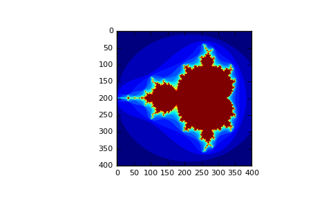 [0, 0, 0, 0]])

你可以参考曼德博集合示例看看如何使用布尔索引来生成曼德博集合的图像。

>>> import numpy as np >>> import matplotlib.pyplot as plt >>> def mandelbrot( h,w, maxit=20 ): ...  """Returns an image of the Mandelbrot fractal of size (h,w).""" ...  y,x = np.ogrid[ -1.4:1.4:h*1j, -2:0.8:w*1j ] ...  c = x+y*1j ...  z = c ...  divtime = maxit + np.zeros(z.shape, dtype=int) ... ...  for i in range(maxit): ...  z = z**2 + c ...  diverge = z*np.conj(z) > 2**2 # who is diverging ...  div_now = diverge & (divtime==maxit) # who is diverging now ...  divtime[div_now] = i # note when ...  z[diverge] = 2 # avoid diverging too much ... ...  return divtime >>> plt.imshow(mandelbrot(400,400)) >>> plt.show()

第二种通过布尔来索引的方法更近似于整数索引；对数组的每个维度我们给一个一维布尔数组来选择我们想要的切片。

>>> a = np.arange(12).reshape(3,4) >>> b1 = np.array([False,True,True]) # first dim selection >>> b2 = np.array([True,False,True,False]) # second dim selection >>> >>> a[b1,:] # selecting rows array([[ 4, 5, 6, 7], [ 8, 9, 10, 11]]) >>> >>> a[b1] # same thing array([[ 4, 5, 6, 7], [ 8, 9, 10, 11]]) >>> >>> a[:,b2] # selecting columns array([[ 0, 2], [ 4, 6], [ 8, 10]]) >>> >>> a[b1,b2] # a weird thing to do array([ 4, 10])

注意一维数组的长度必须和你想要切片的维度或轴的长度一致，在之前的例子中，b1是一个秩为1长度为三的数组(a的行数)，b2(长度为4)与a的第二秩(列)相一致。⁷

ix_()函数

ix_函数可以为了获得多元组的结果而用来结合不同向量。例如，如果你想要用所有向量a、b和c元素组成的三元组来计算a+b*c：

>>> a = np.array([2,3,4,5]) >>> b = np.array([8,5,4]) >>> c = np.array([5,4,6,8,3]) >>> ax,bx,cx = np.ix_(a,b,c) >>> ax array([[[2]], [[3]], [[4]], [[5]]]) >>> bx array([[[8], [5], [4]]]) >>> cx array([[[5, 4, 6, 8, 3]]]) >>> ax.shape, bx.shape, cx.shape ((4, 1, 1), (1, 3, 1), (1, 1, 5)) >>> result = ax+bx*cx >>> result array([[[42, 34, 50, 66, 26], [27, 22, 32, 42, 17], [22, 18, 26, 34, 14]], [[43, 35, 51, 67, 27], [28, 23, 33, 43, 18], [23, 19, 27, 35, 15]], [[44, 36, 52, 68, 28], [29, 24, 34, 44, 19], [24, 20, 28, 36, 16]], [[45, 37, 53, 69, 29], [30, 25, 35, 45, 20], [25, 21, 29, 37, 17]]]) >>> result[3,2,4] 17 >>> a[3]+b[2]*c[4] 17

你也可以实行如下简化：

def ufunc_reduce(ufct, *vectors): vs = np.ix_(*vectors) r = ufct.identity for v in vs: r = ufct(r,v) return r

然后这样使用它：

>>> ufunc_reduce(np.add,a,b,c) array([[[15, 14, 16, 18, 13], [12, 11, 13, 15, 10], [11, 10, 12, 14, 9]], [[16, 15, 17, 19, 14], [13, 12, 14, 16, 11], [12, 11, 13, 15, 10]], [[17, 16, 18, 20, 15], [14, 13, 15, 17, 12], [13, 12, 14, 16, 11]], [[18, 17, 19, 21, 16], [15, 14, 16, 18, 13], [14, 13, 15, 17, 12]]])

这个reduce与ufunc.reduce(比如说add.reduce)相比的优势在于它利用了广播法则，避免了创建一个输出大小乘以向量个数的参数数组。⁸

用字符串索引

参见RecordArray。

线性代数

继续前进，基本线性代数包含在这里。

简单数组运算

参考numpy文件夹中的linalg.py获得更多信息

>>> import numpy as np >>> a = np.array([[1.0, 2.0], [3.0, 4.0]]) >>> print(a) [[ 1. 2.] [ 3. 4.]] >>> a.transpose() array([[ 1., 3.], [ 2., 4.]]) >>> np.linalg.inv(a) array([[-2. , 1. ], [ 1.5, -0.5]]) >>> u =np.eye(2) # unit 2x2 matrix; "eye" represents "I" >>> u array([[ 1., 0.], [ 0., 1.]]) >>> j = np.array([[0.0, -1.0], [1.0, 0.0]]) >>> np.dot (j, j) # matrix product array([[-1., 0.], [ 0., -1.]]) >>> np.trace(u) # trace 2.0 >>> y = np.array([[5.], [7.]]) >>> np.linalg.solve(a, y) array([[-3.], [ 4.]]) >>> np.linalg.eig(j) (array([ 0.+1.j, 0.-1.j]), array([[ 0.70710678+0.j, 0.70710678+0.j], [ 0.00000000-0.70710678j, 0.00000000+0.70710678j]])) Parameters: square matrix Returns The eigenvalues, each repeated according to its multiplicity. The normalized (unit "length") eigenvectors, such that the column ``v[:,i]`` is the eigenvector corresponding to the eigenvalue ``w[i]`` .

技巧和提示

下面我们给出简短和有用的提示。

“自动”改变形状

更改数组的维度，你可以省略一个尺寸，它将被自动推导出来。

>>> a = np.arange(30) >>> a.shape = 2,-1,3 # -1 means "whatever is needed" >>> a.shape (2, 5, 3) >>> a array([[[ 0, 1, 2], [ 3, 4, 5], [ 6, 7, 8], [ 9, 10, 11], [12, 13, 14]], [[15, 16, 17], [18, 19, 20], [21, 22, 23], [24, 25, 26], [27, 28, 29]]])

向量组合(stacking)

我们如何用两个相同尺寸的行向量列表构建一个二维数组？在MATLAB中这非常简单：如果x和y是两个相同长度的向量，你仅仅需要做m=[x;y]。在NumPy中这个过程通过函数column_stack、dstack、hstack和vstack来完成，取决于你想要在那个维度上组合。例如：

x = np.arange(0,10,2) # x=([0,2,4,6,8]) y = np.arange(5) # y=([0,1,2,3,4]) m = np.vstack([x,y]) # m=([[0,2,4,6,8], # [0,1,2,3,4]]) xy = np.hstack([x,y]) # xy =([0,2,4,6,8,0,1,2,3,4])

二维以上这些函数背后的逻辑会很奇怪。

参考写个Matlab用户的NumPy指南并且在这里添加你的新发现: )

直方图(histogram)

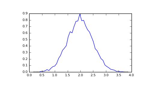
NumPy中histogram函数应用到一个数组返回一对变量：直方图数组和箱式向量。注意：matplotlib也有一个用来建立直方图的函数(叫作hist,正如matlab中一样)与NumPy中的不同。主要的差别是pylab.hist自动绘制直方图，而numpy.histogram仅仅产生数据。

import numpy as np import matplotlib.pyplot as plt # Build a vector of 10000 normal deviates with variance 0.5^2 and mean 2 mu, sigma = 2, 0.5 v =np.random.normal(mu,sigma,10000) # Plot a normalized histogram with 50 bins plt.hist(v, bins=50, normed=1) # matplotlib version (plot) pylab.show() # Compute the histogram with numpy and then plot it (n, bins) = numpy.histogram(v, bins=50, normed=True) # NumPy version (no plot) plt.plot(.5*(bins[1:]+bins[:-1]), n) plt.show()