撰文 | BBuf
原文首发于公众号GiantPandaCV
这篇文章基于自己为OneFlow框架开发 interpolate 这个Op总结而来,OneFlow的 interpolate Op 和 Pytorch的功能一致,都是用来实现插值上采样或者下采样的。在实现这个Op的时候还给Pytorch修复了一个bug并合并到了主仓库,见:
https://github.com/pytorch/pytorch/commit/6ab3a210983b7eee417e7cd92a8ad2677065e470 。因此OneFlow框架中的 interpolate 算子和Pytorch中的 interpolate 算子的功能是完全等价的。这篇文章就以OneFlow中这个算子的实现为例来盘点一下深度学习框架中的那些插值算法。
1 doc && interface接口
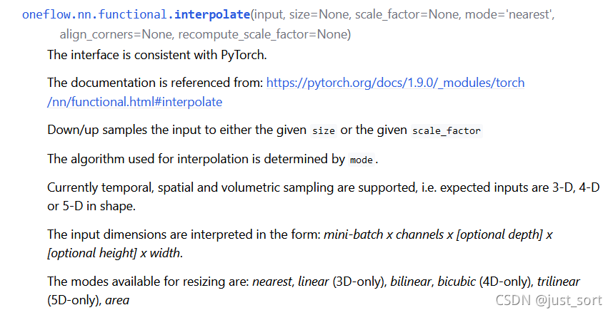
要了解 interpolate 算子中的插值需要 算法,首先 从文档和Python前端接口看起。 看一下接口文档,https://oneflow.readthedocs.io/en/master/functional.html?highlight=interpolate 。
功能介绍
这里可以看到OneFlow的 interpolate 算子用来实现插值上采样或者下采样的功能,支持3-D,4-D,5-D的输入Tensor,然后提供了多种插值的方式应用于不同Shape的输入Tensor。下面再看一下参数列表:
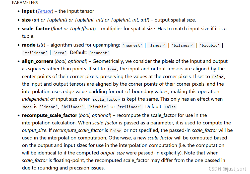
参数列表
size :插值后输出Tensor的空间维度的大小,这个spatial size就是去掉Batch,Channel,Depth维度后剩下的值。比如NCHW的spatial size是HW。
scale_factor (float 或者 Tuple[float]):spatial size的乘数,如果是tuple则必须匹配输入数据的大小。
mode (str):上采样的模式,包含'nearest' | 'linear' | 'bilinear' | 'bicubic' | 'trilinear' | 'area'。默认是 'nearest'。
align_corners (bool):在几何上,我们将输入和输出的像素视为正方形而不是点。如果设置为 True ,则输入和输出张量按其角像素的中心点对齐,保留角像素处的值。如果设置为 False ,则输入和输出张量按其角像素的角点对齐,插值使用边缘值填充来处理边界外值,当 scale_factor 保持不变时,此操作与输入大小无关。这仅在 mode 为 'linear' | 'bilinear' | 'bicubic' | 'trilinear'时有效。默认值是 False 。(没看懂没关系,下面有一节专门讲解)
recompute_scale_factor (bool):重新计算用于插值计算的 scale_factor。当 scale_factor 作为参数传递时,它用于计算 output_size。如果 recompute_scale_factor 为 False 或未指定,则传入的 scale_factor 将用于插值计算。否则,将根据用于插值计算的输出和输入大小计算新的 scale_factor(即,等价于显示传入 output_size )。请注意,当 scale_factor 是浮点数时,由于舍入和精度问题,重新计算的 scale_factor 可能与传入的不同。
除了功能描述和参数描述之外还有几个注意事项和warning,大家可以自行查看文档。下面贴一段如何使用的示例代码,非常简单。
>>> import oneflow as flow>>> import numpy as np>>> input = flow.Tensor(np.arange(1 , 5 ).reshape((1 , 1 , 4 )), dtype=flow.float32)>>> output = flow.nn.functional.interpolate(input, scale_factor=2.0 , mode="linear" )>>> output1.0000 , 1.2500 , 1.7500 , 2.2500 , 2.7500 , 3.2500 , 3.7500 , 4.0000 ]]], 介绍完文档之后,我们看一下这个Op实现的Python前端接口,代码见: https://github.com/Oneflow-Inc/oneflow/blob/master/python/oneflow/nn/modules/interpolate.py#L25-L193 。这里的主要逻辑就是在根据是否传入了 recompute_scale_factor 参数来重新计算 scale_factor 的值,在获得了 scale_factor 之后根据传入的 mode 调用不同的插值Kernel的实现。见:
if len(x.shape) == 3 and self.mode == "nearest" :return flow._C.upsample_nearest_1d(0 ], data_format="channels_first" if len(x.shape) == 4 and self.mode == "nearest" :return flow._C.upsample_nearest_2d(0 ],1 ],"channels_first" ,if len(x.shape) == 5 and self.mode == "nearest" :return flow._C.upsample_nearest_3d(0 ],1 ],2 ],"channels_first" ,if len(x.shape) == 3 and self.mode == "area" :assert output_size is not None return flow._C.adaptive_avg_pool1d(x, output_size)if len(x.shape) == 4 and self.mode == "area" :assert output_size is not None return flow._C.adaptive_avg_pool2d(x, output_size)if len(x.shape) == 5 and self.mode == "area" :assert output_size is not None return flow._C.adaptive_avg_pool3d(x, output_size)if len(x.shape) == 3 and self.mode == "linear" :assert self.align_corners is not None return flow._C.upsample_linear_1d(0 ],"channels_first" ,if len(x.shape) == 4 and self.mode == "bilinear" :assert self.align_corners is not None return flow._C.upsample_bilinear_2d(0 ],1 ],"channels_first" ,if len(x.shape) == 4 and self.mode == "bicubic" :assert self.align_corners is not None return flow._C.upsample_bicubic_2d(0 ],1 ],"channels_first" ,if len(x.shape) == 5 and self.mode == "trilinear" :assert self.align_corners is not None return flow._C.upsample_trilinear_3d(0 ],1 ],2 ],"channels_first" , 所以Python前端就是处理了一些参数关系,然后调用了C++层的API来完成真正的计算过程。下面我们将分别介绍各种插值算法的原理以及在OneFlow中的实现。
2 AlignCorners解释 在上面的接口中, align_corners 是一个非常重要的参数,这里我们先解释一下这个参数是什么含义再继续讲解每种Kernel的实现。这里以一张图片的nearest插值为例讲解align_corners的具体含义。
假设原始图像的大小是
,目标图像是
,那么两幅图像的边长比分别是
和
。那么目标图像的
位置的像素可以通过上面的边长比对应回原图像,坐标为
,那么最近的四个像素是
,
,
,
,
,
,
。如果图形是灰度图,那么
点的像素值可以通过下面的公式计算:其中,
为最近的
个像素点,
为各点的权重。
到这里并没有结束,我们需要特别注意的是,仅仅按照上面得到公式实现的双线性插值的结果和OpenCV/Matlab的结果是对应不起来的,这是为什么呢?
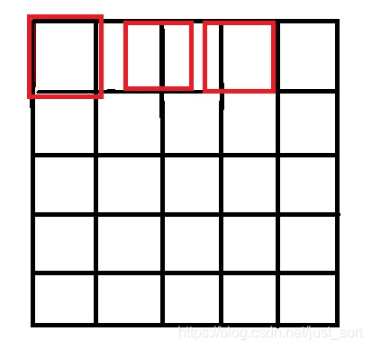
原因就是因为坐标系的选取问题,按照一些网上的公开实现,将源图像和目标图像的原点均选在左上角,然后根据插值公式计算目标图像每个点的像素,假设我们要将
的图像缩小成
,那么源图像和目标图像的对应关系如下图所示:
按照网上大多数公开的源码实现的像素对应关系
可以看到如果选择了左上角作为原点,那么最右边和最下边的像素是没有参与计算的,所以我们得到的结果和OpenCV/MatLab中的结果不会一致,那应该怎么做才是对的呢?
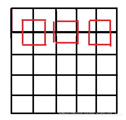
答案就是让两个图像的几何中心重合,并且目标图像的每个像素之间都是等间隔的,并且都和两边有一定的边距 。如下图所示:
让两个图像的几何中心重合后的像素对应关系
int x=(i+0.5 )*m/a-0.5 ;int y=(j+0.5 )*n/b-0.5 ; 所以在 interpolate Op的实现中提供了 align_corners 这个参数让用户选择是否对齐输入和输出的几何中心。
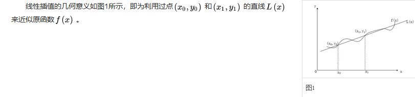
3 Linear插值 Linaer插值即线性插值。线性插值的几何意义即为概述图中利用过A点和B点的直线来近似表示原函数。如下图所示:
Linear插值的几何意义
在OneFlow中实现线性插值的代码在 https://github.com/Oneflow-Inc/oneflow/blob/master/oneflow/user/kernels/upsample_linear_1d_kernel.cpp ,我们只看前向,代码中的 h1lambda 就对应了这个公式里面的
。
template <typename T>GetLinearInputIndex (const int64_t out_dim_idx, const T scale, bool align_corners) if (align_corners) {return static_cast <T>(scale * out_dim_idx);else {0.5 ) - 0.5 ;return static_cast <T>(src_idx < 0 ? 0 : src_idx);static void UpsampleLinear1DForward (const int64_t elem_cnt, const T* in_dptr,int64_t , 3 > in_helper,int64_t , 3 > out_helper, const int in_height,const float scale_factor, bool align_corners, T* out_dptr) for (int64_t index = 0 ; index < elem_cnt; ++index) {int64_t n, c, h;const T h1r = GetLinearInputIndex(h, scale_factor, align_corners);const int64_t h1 = h1r;const int64_t h1p = (h1 < in_height - 1 ) ? 1 : 0 ;const T h1lambda = h1r - h1;const T h0lambda = static_cast <T>(1. ) - h1lambda; 线性邻插值支持输入Tensor为3-D(NCW)。
4 nearest插值 最近邻插值法在放大图像时补充的像素是最近邻的像素的值。在0x2中已经讲解了最近邻插值的做法,假设原始图像的大小是
,目标图像是
,那么两幅图像的边长比分别是
和
。那么目标图像的
位置的像素可以通过上面的边长比对应回原图像,坐标为这种插值缺点就是会导致像素的变化不连续,在新图中会产生锯齿 。
在OneFlow中实现最近邻插值的代码在 https://github.com/Oneflow-Inc/oneflow/blob/master/oneflow/user/kernels/upsample_nearest_kernel.cpp ,这里以输入Tensor为NCW为例代码如下:
OF_DEVICE_FUNC static int64_t GetNearestInputIndex (const int64_t out_dim_idx, const float scale,const int64_t in_dim_size) {int64_t index = static_cast <int64_t >(std ::floor ((static_cast <float >(out_dim_idx) * scale)));1 ? in_dim_size - 1 : index;static_cast <int64_t >(0 ) ? static_cast <int64_t >(0 ) : index;return index;template <typename T>static void UpsampleNearest1DForward (const int64_t elem_cnt, const T* in_dptr,int64_t , 3 > in_helper,int64_t , 3 > out_helper,const int64_t in_height, const float scale_factor, for (int64_t index = 0 ; index < elem_cnt; ++index) {int64_t n, c, h;const int64_t in_h = GetNearestInputIndex(h, scale_factor, in_height); 最近邻插值支持输入Tensor为3-D(NCW),4-D(NCHW),5-D(NCDHW)。
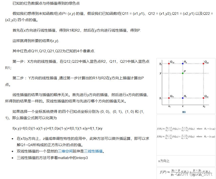
6 bilinear插值 假设原始图像的大小是
,目标图像是
,那么两幅图像的边长比分别是
和
。那么目标图像的
位置的像素可以通过上面的边长比对应回原图像,坐标为
,那么最近的四个像素是
,
,
,
,
,
,
。如果图形是灰度图,那么
点的像素值可以通过下面的公式计算:。其中,
为最近的
个像素点,
为各点的权重。
双线性插值原理
按照上面的方法来实现代码,OneFlow中实现在 https://github.com/Oneflow-Inc/oneflow/blob/master/oneflow/user/kernels/upsample_bilinear_2d_kernel.cpp ,这里只看前向:
template <typename T>void GetBilinearParam (const bool align_corners, const int64_t h, const int64_t w,const int64_t in_height, const int64_t in_width,const T scale_h, const T scale_w, BilinearParam<T>* params) if (align_corners) {static_cast <T>(h);else {static_cast <T>(h) + 0.5f ) * scale_h - 0.5f ;0 ? 0 : h1r;const int64_t h1 = h1r;const int64_t h1p = (h1 < in_height - 1 ) ? 1 : 0 ;if (align_corners) {static_cast <T>(w);else {static_cast <T>(w) + 0.5f ) * scale_w - 0.5f ;0 ? 0 : w1r;const int64_t w1 = w1r;const int64_t w1p = (w1 < in_width - 1 ) ? 1 : 0 ;template <typename T>static void UpsampleBilinear2DForward (const int64_t elem_cnt, const T* in_dptr,int64_t , 4 > in_helper,int64_t , 4 > out_helper,const int64_t in_height, const int64_t in_width,const T scale_h, const T scale_w, const bool align_corners, for (int64_t index = 0 ; index < elem_cnt; ++index) {int64_t n, c, h, w;const int64_t top_offset = in_helper.NdIndexToOffset(n, c, params.top_h_index, 0 );const int64_t bottom_offset = in_helper.NdIndexToOffset(n, c, params.bottom_h_index, 0 );const T top_left = in_dptr[top_offset + params.left_w_index];const T top_right = in_dptr[top_offset + params.right_w_index];const T bottom_left = in_dptr[bottom_offset + params.left_w_index];const T bottom_right = in_dptr[bottom_offset + params.right_w_index];const T top = top_left + (top_right - top_left) * params.w_lerp;const T bottom = bottom_left + (bottom_right - bottom_left) * params.w_lerp; 和上面图片中的过程是一一对应的。双线性插值相对于最近邻插值好处就是目标像素是由原始图像中多个像素插值来的,图形就会比较平滑,不会产生锯齿。
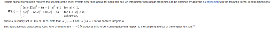
6 bicubic 插值 双三次插值是一种更加复杂的插值方式,它能创造出比双线性插值更平滑的图像边缘。
wiki:在数值分析这个数学分支中,双三次插值(英语:Bicubic interpolation)是二维空间中最常用的插值方法。在这种方法中,函数 f 在点 (x, y) 的值可以通过矩形网格中最近的十六个采样点的加权平均得到,在这里需要使用两个多项式插值三次函数,每个方向使用一个。
这是实现 interpolate 这个算子时最复杂的一种插值方式,计算过程如下:
bicubic插值公式
bicubic插值权重的计算方法
注意这里提到
一般取-0.5或者-0.75,我们这里和Pytorch以及OpenCV保持一致,取-0.75。计算W的过程代码实现如下:
// Based on // https://en.wikipedia.org/wiki/Bicubic_interpolation#Bicubic_convolution_algorithm template <typename T>cubic_convolution1 (const T x, const T A) return ((A + 2.0 ) * x - (A + 3.0 )) * x * x + 1.0 ;template <typename T>cubic_convolution2 (const T x, const T A) return ((A * x - 5.0 * A) * x + 8.0 * A) * x - 4.0 * A;template <typename T>void get_cubic_upsample_coefficients (T coeffs[4 ], const T t) -0.75 ;0 ] = cubic_convolution2<T>(x1 + 1.0 , A);1 ] = cubic_convolution1<T>(x1, A);// opposite coefficients 1.0 - t;2 ] = cubic_convolution1<T>(x2, A);3 ] = cubic_convolution2<T>(x2 + 1.0 , A);template <typename T>cubic_interp1d (const T x0, const T x1, const T x2, const T x3, const T t) 4 ];return x0 * coeffs[0 ] * 1.0 + x1 * coeffs[1 ] * 1.0 + x2 * coeffs[2 ] * 1.0 + x3 * coeffs[3 ] * 1.0 ;
void Compute (user_op::KernelComputeContext* ctx) const override const user_op::Tensor* x_tensor = ctx->Tensor4ArgNameAndIndex("x" , 0 );"y" , 0 );const T* in_ptr = x_tensor->dptr<T>();const float height_scale = ctx->Attr<float >("height_scale" );const float width_scale = ctx->Attr<float >("width_scale" );const bool align_corners = ctx->Attr<bool >("align_corners" );const int nbatch = x_tensor->shape().At(0 );const int channels = x_tensor->shape().At(1 );const int64_t in_height = x_tensor->shape().At(2 );const int64_t in_width = x_tensor->shape().At(3 );const int64_t out_height = y_tensor->shape().At(2 );const int64_t out_width = y_tensor->shape().At(3 );if (in_height == out_height && in_width == out_width) {memcpy (out_ptr, in_ptr, sizeof (T) * nbatch * channels * in_height * in_width);else {const T scale_height = GetAreaPixelScale(in_height, out_height, align_corners, height_scale);const T scale_width = GetAreaPixelScale(in_width, out_width, align_corners, width_scale);for (int64_t output_y = 0 ; output_y < out_height; output_y++) {for (int64_t output_x = 0 ; output_x < out_width; output_x++) {const T* in = in_ptr;const T real_x = GetAreaPixel(scale_width, output_x, align_corners, /*cubic=*/ true );int64_t input_x = std ::floor (real_x);const T t_x = real_x - input_x;const T real_y = GetAreaPixel(scale_height, output_y, align_corners, /*cubic=*/ true );int64_t input_y = std ::floor (real_y);const T t_y = real_y - input_y;for (int64_t c = 0 ; c < channels * nbatch; c++) {4 ];// Interpolate 4 times in the x direction for (int64_t i = 0 ; i < 4 ; i++) {1 , input_y - 1 + i),0 , input_y - 1 + i),1 , input_y - 1 + i),2 , input_y - 1 + i),// Interpolate in the y direction using x interpolations 0 ], coefficients[1 ], coefficients[2 ], coefficients[3 ], t_y);// Move to next channel 从代码可以看到,这里的一次2维bicubic插值被拆成了2次1维的bicubic插值。
bicubic插值支持4维(NCHW)的输入数据,插值后的图形比bilinear更加精细平滑 。
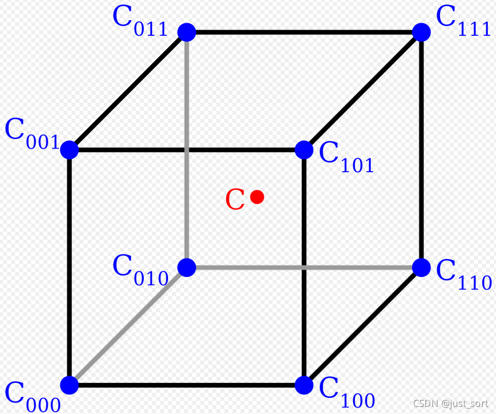
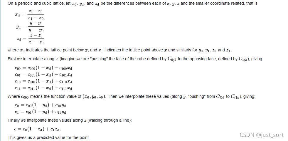
7 trilinear插值 三线性插值(trilinear interpolation)主要是用于在一个3D的立方体中,通过给定顶点的数值然后计算立方体中其他点的数值的线性插值方法。如下图:
三线性插值示意图
首先我们需要选择一个方向,然后线性插值一次将其变成双线性插值,这样就可以套用上面双线性的公式了。我在实现的时候为了简单直接选择了wiki百科给出的最终公式:
trilinear插值的原理和实现过程
在OneFlow中代码实现在这里: https://github.com/Oneflow-Inc/oneflow/blob/master/oneflow/user/kernels/upsample_trilinear_3d_kernel.cpp#L25-L69 ,这里只看前向:
template <typename T>static void UpsampleTrilinear3DForward (const int64_t elem_cnt, const T* in_dptr,int64_t , 5 > in_helper,int64_t , 5 > out_helper,const int64_t in_depth, const int64_t in_height,const int64_t in_width, const T rdepth, const T rheight,const T rwidth, const bool align_corners, T* out_dptr) for (int64_t index = 0 ; index < elem_cnt; ++index) {int64_t n, c, d, h, w;const T t1r = GetAreaPixel(rdepth, d, align_corners);const int64_t t1 = t1r;const int64_t t1p = (t1 < in_depth - 1 ) ? 1 : 0 ;const T t1lambda = t1r - t1;const T t0lambda = static_cast <T>(1. ) - t1lambda;const T h1r = GetAreaPixel(rheight, h, align_corners);const int64_t h1 = h1r;const int64_t h1p = (h1 < in_height - 1 ) ? 1 : 0 ;const T h1lambda = h1r - h1;const T h0lambda = static_cast <T>(1. ) - h1lambda;const T w1r = GetAreaPixel(rwidth, w, align_corners);const int64_t w1 = w1r;const int64_t w1p = (w1 < in_width - 1 ) ? 1 : 0 ;const T w1lambda = w1r - w1;const T w0lambda = static_cast <T>(1. ) - w1lambda;const T* pos1 = &in_dptr[in_helper.NdIndexToOffset(n, c, t1, h1, w1)];0 ] + w1lambda * pos1[w1p]) 上面的代码对应了trilinear插值的实现过程,将其分别为三次独立的线性插值。
trilinear插值支持5维(NCDHW)输入数据。
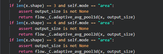
8 area插值
interpolate 算子中还有一种插值方法,即 area 插值,代码如下:
area插值即adaptive_avg_pool
可以看到area插值就是adaptive_avg_pool,自适应平均池化。由于自适应平均池化中一个输出像素对应了一个区域的输入像素所以插值的mode参数为 area ,这样想比较好理解。关于adaptive_avg_pool的细节我就不讲了,思路就是枚举输出像素然后找到对应的输入像素的区域进行像素求和和取平均。感兴趣可以看一下OneFlow的具体实现: https://github.com/Oneflow-Inc/oneflow/blob/master/oneflow/user/kernels/adaptive_pool_cpu_kernel.cpp
9 插值方法比较 上面介绍了 interpolate Op的各种插值算法,从Nearest到BiLinear再到Bicubic,获得的结果越来越平滑,但计算的代价也相应的增大。OneFlow和Pytorch一样将基于这个实现各种Upsample Module。还需要说明的是上采样除了这个 interpolate 中提到的方法还有反卷积方法,之前已经讲过了,这里就不重复补充。
另外上面介绍的示例代码都是CPU版本,只需要在对应链接下找同名的.cu文件就可以看到GPU版本的代码。
本文以 interpolate 算子的开发过程为例,梳理了深度学习框架中基本所有的插值方法,希望可以帮助到读者。
点击“ 阅读原文 ” ,欢迎下载体验OneFlow新一代开源深度学习框架