Pandas提供快速,灵活和富于表现力的数据结构,是强大的数据分析Python库。
本文收录于机器学习前置教程系列。
一、Series和DataFrame
Pandas建立在NumPy之上,更多NumPy相关的知识点可以参考我之前写的文章前置机器学习(三):30分钟掌握常用NumPy用法。
Pandas特别适合处理表格数据,如SQL表格、EXCEL表格。有序或无序的时间序列。具有行和列标签的任意矩阵数据。
打开Jupyter Notebook,导入numpy和pandas开始我们的教程:
import numpy as np
import pandas as pd
1. pandas.Series
Series是带有索引的一维ndarray数组。索引值可不唯一,但必须是可哈希的。
pd.Series([1, 3, 5, np.nan, 6, 8])
输出:
0    1.0
1    3.0
2    5.0
3    NaN
4    6.0
5    8.0
dtype: float64
我们可以看到默认索引值为0、1、2、3、4、5这样的数字。添加index属性,指定其为'c','a','i','yong','j','i'。
pd.Series([1, 3, 5, np.nan, 6, 8], index=['c','a','i','yong','j','i'])
输出如下,我们可以看到index是可重复的。
c       1.0
a       3.0
i       5.0
yong    NaN
j       6.0
i       8.0
dtype: float64
2. pandas.DataFrame
DataFrame是带有行和列的表格结构。可以理解为多个Series对象的字典结构。
pd.DataFrame(np.array([[1, 2, 3], [4, 5, 6], [7, 8, 9]]), index=['i','ii','iii'], columns=['A', 'B', 'C'])
输出表格如下,其中index对应它的行,columns对应它的列。
|
A |
B |
C |
| i |
1 |
2 |
3 |
| ii |
4 |
5 |
6 |
| iii |
7 |
8 |
9 |
二、Pandas常见用法
1. 访问数据
准备数据,随机生成6行4列的二维数组,行标签为从20210101到20210106的日期,列标签为A、B、C、D。
import numpy as np
import pandas as pd
np.random.seed(20201212)
df = pd.DataFrame(np.random.randn(6, 4), index=pd.date_range('20210101', periods=6), columns=list('ABCD'))
df
展示表格如下:
|
A |
B |
C |
D |
| 2021-01-01 |
0.270961 |
-0.405463 |
0.348373 |
0.828572 |
| 2021-01-02 |
0.696541 |
0.136352 |
-1.64592 |
-0.69841 |
| 2021-01-03 |
0.325415 |
-0.602236 |
-0.134508 |
1.28121 |
| 2021-01-04 |
-0.33032 |
-1.40384 |
-0.93809 |
1.48804 |
| 2021-01-05 |
0.348708 |
1.27175 |
0.626011 |
-0.253845 |
| 2021-01-06 |
-0.816064 |
1.30197 |
0.656281 |
-1.2718 |
1.1 head()和tail()
查看表格前几行:
df.head(2)
展示表格如下:
|
A |
B |
C |
D |
| 2021-01-01 |
0.270961 |
-0.405463 |
0.348373 |
0.828572 |
| 2021-01-02 |
0.696541 |
0.136352 |
-1.64592 |
-0.69841 |
查看表格后几行:
df.tail(3)
展示表格如下:
|
A |
B |
C |
D |
| 2021-01-04 |
-0.33032 |
-1.40384 |
-0.93809 |
1.48804 |
| 2021-01-05 |
0.348708 |
1.27175 |
0.626011 |
-0.253845 |
| 2021-01-06 |
-0.816064 |
1.30197 |
0.656281 |
-1.2718 |
1.2 describe()
describe方法用于生成DataFrame的描述统计信息。可以很方便的查看数据集的分布情况。注意,这里的统计分布不包含NaN值。
df.describe()
展示如下:
|
A |
B |
C |
D |
| count |
6 |
6 |
6 |
6 |
| mean |
0.0825402 |
0.0497552 |
-0.181309 |
0.22896 |
| std |
0.551412 |
1.07834 |
0.933155 |
1.13114 |
| min |
-0.816064 |
-1.40384 |
-1.64592 |
-1.2718 |
| 25% |
-0.18 |
-0.553043 |
-0.737194 |
-0.587269 |
| 50% |
0.298188 |
-0.134555 |
0.106933 |
0.287363 |
| 75% |
0.342885 |
0.987901 |
0.556601 |
1.16805 |
| max |
0.696541 |
1.30197 |
0.656281 |
1.48804 |
我们首先回顾一下我们掌握的数学公式。
平均数(mean):
$$\bar x = \frac{\sum_{i=1}^{n}{x_i}}{n}$$
方差(variance):
$$s^2 = \frac{\sum_{i=1}^{n}{(x_i -\bar x)^2}}{n}$$
标准差(std):
$$s = \sqrt{\frac{\sum_{i=1}^{n}{(x_i -\bar x)^2}}{n}}$$
我们解释一下pandas的describe统计信息各属性的意义。我们仅以 A 列为例。
count表示计数。A列有6个数据不为空。mean表示平均值。A列所有不为空的数据平均值为0.0825402。std表示标准差。A列的标准差为0.551412。min表示最小值。A列最小值为-0.816064。即,0%的数据比-0.816064小。25%表示四分之一分位数。A列的四分之一分位数为-0.18。即,25%的数据比-0.18小。50%表示二分之一分位数。A列的四分之一分位数为0.298188。即,50%的数据比0.298188小。75%表示四分之三分位数。A列的四分之三分位数为0.342885。即,75%的数据比0.342885小。max表示最大值。A列的最大值为0.696541。即,100%的数据比0.696541小。
1.3 T
T一般表示Transpose的缩写,即转置。行列转换。
df.T
展示表格如下:
|
2021-01-01 |
2021-01-02 |
2021-01-03 |
2021-01-04 |
2021-01-05 |
2021-01-06 |
| A |
0.270961 |
0.696541 |
0.325415 |
-0.33032 |
0.348708 |
-0.816064 |
| B |
-0.405463 |
0.136352 |
-0.602236 |
-1.40384 |
1.27175 |
1.30197 |
| C |
0.348373 |
-1.64592 |
-0.134508 |
-0.93809 |
0.626011 |
0.656281 |
| D |
0.828572 |
-0.69841 |
1.28121 |
1.48804 |
-0.253845 |
-1.2718 |
1.4 sort_values()
指定某一列进行排序,如下代码根据C列进行正序排序。
df.sort_values(by='C')
展示表格如下:
|
A |
B |
C |
D |
| 2021-01-02 |
0.696541 |
0.136352 |
-1.64592 |
-0.69841 |
| 2021-01-04 |
-0.33032 |
-1.40384 |
-0.93809 |
1.48804 |
| 2021-01-03 |
0.325415 |
-0.602236 |
-0.134508 |
1.28121 |
| 2021-01-01 |
0.270961 |
-0.405463 |
0.348373 |
0.828572 |
| 2021-01-05 |
0.348708 |
1.27175 |
0.626011 |
-0.253845 |
| 2021-01-06 |
-0.816064 |
1.30197 |
0.656281 |
-1.2718 |
1.5 nlargest()
选择某列最大的n行数据。如:df.nlargest(2,'A')表示,返回A列最大的2行数据。
df.nlargest(2,'A')
展示表格如下:
|
A |
B |
C |
D |
| 2021-01-02 |
0.696541 |
0.136352 |
-1.64592 |
-0.69841 |
| 2021-01-05 |
0.348708 |
1.27175 |
0.626011 |
-0.253845 |
1.6 sample()
sample方法表示查看随机的样例数据。
df.sample(5)表示返回随机5行数据。
df.sample(5)
参数frac表示fraction,分数的意思。frac=0.01即返回1%的随机数据作为样例展示。
df.sample(frac=0.01)
2. 选择数据
2.1 根据标签选择
我们输入df['A']命令选取A列。
df['A']
输出A列数据,同时也是一个Series对象:
2021-01-01    0.270961
2021-01-02    0.696541
2021-01-03    0.325415
2021-01-04   -0.330320
2021-01-05    0.348708
2021-01-06   -0.816064
Name: A, dtype: float64
df[0:3]该代码与df.head(3)同理。但df[0:3]是NumPy的数组选择方式,这说明了Pandas对于NumPy具有良好的支持。
df[0:3]
展示表格如下: | | A | B | C | D | |:-----------|---------:|----------:|----------:|----------:| | 2021-01-01 | 0.270961 | -0.405463 | 0.348373 | 0.828572 | | 2021-01-02 | 0.696541 | 0.136352 | -1.64592 | -0.69841 | | 2021-01-03 | 0.325415 | -0.602236 | -0.134508 | 1.28121 |
通过loc方法指定行列标签。
df.loc['2021-01-01':'2021-01-02', ['A', 'B']]
展示表格如下:
|
A |
B |
| 2021-01-01 |
0.270961 |
-0.405463 |
| 2021-01-02 |
0.696541 |
0.136352 |
2.2 根据位置选择
iloc 与loc不同。loc指定具体的标签,而iloc指定标签的索引位置。df.iloc[3:5, 0:3]表示选取索引为3、4的行,索引为0、1、2的列。即,第4、5行,第1、2、3列。 注意,索引序号从0开始。冒号表示区间,左右两侧分别表示开始和结束。如3:5表示左开右闭区间[3,5),即不包含5自身。
df.iloc[3:5, 0:3]
|
A |
B |
C |
| 2021-01-04 |
-0.33032 |
-1.40384 |
-0.93809 |
| 2021-01-05 |
0.348708 |
1.27175 |
0.626011 |
df.iloc[:, 1:3]
|
B |
C |
| 2021-01-01 |
-0.405463 |
0.348373 |
| 2021-01-02 |
0.136352 |
-1.64592 |
| 2021-01-03 |
-0.602236 |
-0.134508 |
| 2021-01-04 |
-1.40384 |
-0.93809 |
| 2021-01-05 |
1.27175 |
0.626011 |
| 2021-01-06 |
1.30197 |
0.656281 |
2.3 布尔索引
DataFrame可根据条件进行筛选,当条件判断True时,返回。当条件判断为False时,过滤掉。
我们设置一个过滤器用来判断A列是否大于0。
filter = df['A'] > 0
filter
输出结果如下,可以看到2021-01-04和2021-01-06的行为False。
2021-01-01     True
2021-01-02     True
2021-01-03     True
2021-01-04    False
2021-01-05     True
2021-01-06    False
Name: A, dtype: bool
我们通过过滤器查看数据集。
df[filter]
# df[df['A'] > 0]
查看表格我们可以发现,2021-01-04和2021-01-06的行被过滤掉了。
|
A |
B |
C |
D |
| 2021-01-01 |
0.270961 |
-0.405463 |
0.348373 |
0.828572 |
| 2021-01-02 |
0.696541 |
0.136352 |
-1.64592 |
-0.69841 |
| 2021-01-03 |
0.325415 |
-0.602236 |
-0.134508 |
1.28121 |
| 2021-01-05 |
0.348708 |
1.27175 |
0.626011 |
-0.253845 |
3. 处理缺失值
准备数据。
df2 = df.copy()
df2.loc[:3, 'E'] = 1.0
f_series = {'2021-01-02': 1.0,'2021-01-03': 2.0,'2021-01-04': 3.0,'2021-01-05': 4.0,'2021-01-06': 5.0}
df2['F'] = pd.Series(f_series)
df2
展示表格如下:
|
A |
B |
C |
D |
F |
E |
| 2021-01-01 |
0.270961 |
-0.405463 |
0.348373 |
0.828572 |
nan |
1 |
| 2021-01-02 |
0.696541 |
0.136352 |
-1.64592 |
-0.69841 |
1 |
1 |
| 2021-01-03 |
0.325415 |
-0.602236 |
-0.134508 |
1.28121 |
2 |
1 |
| 2021-01-04 |
-0.33032 |
-1.40384 |
-0.93809 |
1.48804 |
3 |
nan |
| 2021-01-05 |
0.348708 |
1.27175 |
0.626011 |
-0.253845 |
4 |
nan |
| 2021-01-06 |
-0.816064 |
1.30197 |
0.656281 |
-1.2718 |
5 |
nan |
3.1 dropna()
使用dropna方法清空NaN值。注意:dropa方法返回新的DataFrame,并不会改变原有的DataFrame。
df2.dropna(how='any')
以上代码表示,当行数据有任意的数值为空时,删除。
|
A |
B |
C |
D |
F |
E |
| 2021-01-02 |
0.696541 |
0.136352 |
-1.64592 |
-0.69841 |
1 |
1 |
| 2021-01-03 |
0.325415 |
-0.602236 |
-0.134508 |
1.28121 |
2 |
1 |
3.2 fillna()
使用filna命令填补NaN值。
df2.fillna(df2.mean())
以上代码表示,使用每一列的平均值来填补空缺。同样地,fillna并不会更新原有的DataFrame,如需更新原有DataFrame使用代码df2 = df2.fillna(df2.mean())。
展示表格如下:
|
A |
B |
C |
D |
F |
E |
| 2021-01-01 |
0.270961 |
-0.405463 |
0.348373 |
0.828572 |
3 |
1 |
| 2021-01-02 |
0.696541 |
0.136352 |
-1.64592 |
-0.69841 |
1 |
1 |
| 2021-01-03 |
0.325415 |
-0.602236 |
-0.134508 |
1.28121 |
2 |
1 |
| 2021-01-04 |
-0.33032 |
-1.40384 |
-0.93809 |
1.48804 |
3 |
1 |
| 2021-01-05 |
0.348708 |
1.27175 |
0.626011 |
-0.253845 |
4 |
1 |
| 2021-01-06 |
-0.816064 |
1.30197 |
0.656281 |
-1.2718 |
5 |
1 |
4. 操作方法
4.1 agg()
agg是Aggregate的缩写,意为聚合。
常用聚合方法如下:
- mean(): Compute mean of groups
- sum(): Compute sum of group values
- size(): Compute group sizes
- count(): Compute count of group
- std(): Standard deviation of groups
- var(): Compute variance of groups
- sem(): Standard error of the mean of groups
- describe(): Generates descriptive statistics
- first(): Compute first of group values
- last(): Compute last of group values
- nth() : Take nth value, or a subset if n is a list
- min(): Compute min of group values
- max(): Compute max of group values
df.mean()
返回各列平均值
A    0.082540
B    0.049755
C   -0.181309
D    0.228960
dtype: float64
可通过加参数axis查看行平均值。
df.mean(axis=1)
输出:
2021-01-01    0.260611
2021-01-02   -0.377860
2021-01-03    0.217470
2021-01-04   -0.296053
2021-01-05    0.498156
2021-01-06   -0.032404
dtype: float64
如果我们想查看某一列的多项聚合统计怎么办?
这时我们可以调用agg方法:
df.agg(['std','mean'])['A']
返回结果显示标准差std和均值mean:
std     0.551412
mean    0.082540
Name: A, dtype: float64
对于不同的列应用不同的聚合函数:
df.agg({'A':['max','mean'],'B':['mean','std','var']})
返回结果如下:
|
A |
B |
| max |
0.696541 |
nan |
| mean |
0.0825402 |
0.0497552 |
| std |
nan |
1.07834 |
| var |
nan |
1.16281 |
4.2 apply()
apply()是对方法的调用。 如df.apply(np.sum)表示每一列调用np.sum方法,返回每一列的数值和。
df.apply(np.sum)
输出结果为:
A    0.495241
B    0.298531
C   -1.087857
D    1.373762
dtype: float64
apply方法支持lambda表达式。
df.apply(lambda n: n*2)
|
A |
B |
C |
D |
| 2021-01-01 |
0.541923 |
-0.810925 |
0.696747 |
1.65714 |
| 2021-01-02 |
1.39308 |
0.272704 |
-3.29185 |
-1.39682 |
| 2021-01-03 |
0.65083 |
-1.20447 |
-0.269016 |
2.56242 |
| 2021-01-04 |
-0.66064 |
-2.80768 |
-1.87618 |
2.97607 |
| 2021-01-05 |
0.697417 |
2.5435 |
1.25202 |
-0.50769 |
| 2021-01-06 |
-1.63213 |
2.60393 |
1.31256 |
-2.5436 |
4.3 value_counts()
value_counts方法查看各行、列的数值重复统计。 我们重新生成一些整数数据,来保证有一定的数据重复。
np.random.seed(101)
df3 = pd.DataFrame(np.random.randint(0,9,size = (6,4)),columns=list('ABCD'))
df3
|
A |
B |
C |
D |
| 0 |
1 |
6 |
7 |
8 |
| 1 |
4 |
8 |
5 |
0 |
| 2 |
5 |
8 |
1 |
3 |
| 3 |
8 |
3 |
3 |
2 |
| 4 |
8 |
3 |
7 |
0 |
| 5 |
7 |
8 |
4 |
3 |
调用value_counts()方法。
df3['A'].value_counts()
查看输出我们可以看到 A列的数字8有两个,其他数字的数量为1。
8    2
7    1
5    1
4    1
1    1
Name: A, dtype: int64
4.4 str
Pandas内置字符串处理方法。
names = pd.Series(['andrew','bobo','claire','david','4'])
names.str.upper()
通过以上代码我们将Series中的字符串全部设置为大写。
0    ANDREW
1      BOBO
2    CLAIRE
3     DAVID
4         4
dtype: object
首字母大写:
names.str.capitalize()
输出为:
0    Andrew
1      Bobo
2    Claire
3     David
4         4
dtype: object
判断是否为数字:
names.str.isdigit()
输出为:
0    False
1    False
2    False
3    False
4     True
dtype: bool
字符串分割:
tech_finance = ['GOOG,APPL,AMZN','JPM,BAC,GS']
tickers = pd.Series(tech_finance)
tickers.str.split(',').str[0:2]
以逗号分割字符串,结果为:
0    [GOOG, APPL]
1      [JPM, BAC]
dtype: object
5. 合并
5.1 concat()
concat用来将数据集串联起来。我们先准备数据。
data_one = {'Col1': ['A0', 'A1', 'A2', 'A3'],'Col2': ['B0', 'B1', 'B2', 'B3']}
data_two = {'Col1': ['C0', 'C1', 'C2', 'C3'], 'Col2': ['D0', 'D1', 'D2', 'D3']}
one = pd.DataFrame(data_one)
two = pd.DataFrame(data_two)
使用concat方法将两个数据集串联起来。
pt(pd.concat([one,two]))
得到表格: | | Col1 | Col2 | |---:|:-------|:-------| | 0 | A0 | B0 | | 1 | A1 | B1 | | 2 | A2 | B2 | | 3 | A3 | B3 | | 0 | C0 | D0 | | 1 | C1 | D1 | | 2 | C2 | D2 | | 3 | C3 | D3 |
5.2 merge()
merge相当于SQL操作中的join方法,用于将两个数据集通过某种关系连接起来
registrations = pd.DataFrame({'reg_id':[1,2,3,4],'name':['Andrew','Bobo','Claire','David']})
logins = pd.DataFrame({'log_id':[1,2,3,4],'name':['Xavier','Andrew','Yolanda','Bobo']})
我们根据name来连接两个张表,连接方式为outer。
pd.merge(left=registrations, right=logins, how='outer',on='name')
返回结果为:
|
reg_id |
name |
log_id |
| 0 |
1 |
Andrew |
2 |
| 1 |
2 |
Bobo |
4 |
| 2 |
3 |
Claire |
nan |
| 3 |
4 |
David |
nan |
| 4 |
nan |
Xavier |
1 |
| 5 |
nan |
Yolanda |
3 |
我们注意,how : {'left', 'right', 'outer', 'inner'} 有4种连接方式。表示是否选取左右两侧表的nan值。如left表示保留左侧表中所有数据,当遇到右侧表数据为nan值时,不显示右侧的数据。 简单来说,把left表和right表看作两个集合。
- left表示取左表全部集合+两表交集
- right表示取右表全部集合+两表交集
- outer表示取两表并集
- inner表示取两表交集
6. 分组GroupBy
Pandas中的分组功能非常类似于SQL语句SELECT Column1, Column2, mean(Column3), sum(Column4)FROM SomeTableGROUP BY Column1, Column2。即使没有接触过SQL也没有关系,分组就相当于把表格数据按照某一列进行拆分、统计、合并的过程。
准备数据。
np.random.seed(20201212)
df = pd.DataFrame({'A': ['foo', 'bar', 'foo', 'bar', 'foo', 'bar', 'foo', 'foo'],
                   'B': ['one', 'one', 'two', 'three', 'two', 'two', 'one', 'three'],
                   'C': np.random.randn(8),
                   'D': np.random.randn(8)})
df
可以看到,我们的A列和B列有很多重复数据。这时我们可以根据foo/bar或者one/two进行分组。
|
A |
B |
C |
D |
| 0 |
foo |
one |
0.270961 |
0.325415 |
| 1 |
bar |
one |
-0.405463 |
-0.602236 |
| 2 |
foo |
two |
0.348373 |
-0.134508 |
| 3 |
bar |
three |
0.828572 |
1.28121 |
| 4 |
foo |
two |
0.696541 |
-0.33032 |
| 5 |
bar |
two |
0.136352 |
-1.40384 |
| 6 |
foo |
one |
-1.64592 |
-0.93809 |
| 7 |
foo |
three |
-0.69841 |
1.48804 |
6.1 单列分组
我们应用groupby方法将上方表格中的数据进行分组。
df.groupby('A')
执行上方代码可以看到,groupby方法返回的是一个类型为DataFrameGroupBy的对象。我们无法直接查看,需要应用聚合函数。参考本文4.1节。
<pandas.core.groupby.generic.DataFrameGroupBy object at 0x0000014C6742E248>
我们应用聚合函数sum试试。
df.groupby('A').sum()
展示表格如下:
| A |
C |
D |
| bar |
0.559461 |
-0.724868 |
| foo |
-1.02846 |
0.410533 |
6.2 多列分组
groupby方法支持将多个列作为参数传入。
df.groupby(['A', 'B']).sum()
分组后显示结果如下:
| A |
B |
C |
D |
| bar |
one |
-0.405463 |
-0.602236 |
|
one |
-0.405463 |
-0.602236 |
|
three |
0.828572 |
1.28121 |
|
two |
0.136352 |
-1.40384 |
| foo |
one |
-1.37496 |
-0.612675 |
|
three |
-0.69841 |
1.48804 |
|
two |
1.04491 |
-0.464828 |
6.3 应用多聚合方法
我们应用agg(),将聚合方法数组作为参数传入方法。下方代码根据A分类且只统计C列的数值。
df.groupby('A')['C'].agg([np.sum, np.mean, np.std])
可以看到bar组与foo组各聚合函数的结果如下:
| A |
sum |
mean |
std |
| bar |
0.559461 |
0.186487 |
0.618543 |
| foo |
-1.02846 |
-0.205692 |
0.957242 |
6.4 不同列进行不同聚合统计
下方代码对C、D列分别进行不同的聚合统计,对C列进行求和,对D列进行标准差统计。
df.groupby('A').agg({'C': 'sum', 'D': lambda x: np.std(x, ddof=1)})
输出如下:
| A |
C |
D |
| bar |
0.559461 |
1.37837 |
| foo |
-1.02846 |
0.907422 |
6.5 更多
更多关于Pandas的goupby方法请参考官网:https://pandas.pydata.org/pandas-docs/stable/user_guide/groupby.html
三、Pandas 进阶用法
1. reshape
reshape表示重塑表格。对于复杂表格,我们需要将其转换成适合我们理解的样子,比如根据某些属性分组后进行单独统计。
1.1 stack() 和 unstack()
stack方法将表格分为索引和数据两个部分。索引各列保留,数据堆叠放置。
准备数据。
tuples = list(zip(*[['bar', 'bar', 'baz', 'baz','foo', 'foo', 'qux', 'qux'],
                    ['one', 'two', 'one', 'two','one', 'two', 'one', 'two']]))
index = pd.MultiIndex.from_tuples(tuples, names=['first', 'second'])
根据上方代码,我们创建了一个复合索引。
MultiIndex([('bar', 'one'),
            ('bar', 'two'),
            ('baz', 'one'),
            ('baz', 'two'),
            ('foo', 'one'),
            ('foo', 'two'),
            ('qux', 'one'),
            ('qux', 'two')],
           names=['first', 'second'])
我们创建一个具备复合索引的DataFrame。
np.random.seed(20201212)
df = pd.DataFrame(np.random.randn(8, 2), index=index, columns=['A', 'B'])
df
输出如下:
| A |
B |
C |
D |
| bar |
one |
0.270961 |
-0.405463 |
|
two |
0.348373 |
0.828572 |
| baz |
one |
0.696541 |
0.136352 |
|
two |
-1.64592 |
-0.69841 |
| foo |
one |
0.325415 |
-0.602236 |
|
two |
-0.134508 |
1.28121 |
| qux |
one |
-0.33032 |
-1.40384 |
|
two |
-0.93809 |
1.48804 |
我们执行stack方法。
stacked = df.stack()
stacked
输出堆叠(压缩)后的表格如下。注意:你使用Jupyter Notebook/Lab进行的输出可能和如下结果不太一样。下方输出的各位为了方便在Markdown中显示有一定的调整。
first  second
bar    one     A    0.942502
bar    one     B    0.060742
bar    two     A    1.340975
bar    two     B   -1.712152
baz    one     A    1.899275
baz    one     B    1.237799
baz    two     A   -1.589069
baz    two     B    1.288342
foo    one     A   -0.326792
foo    one     B    1.576351
foo    two     A    1.526528
foo    two     B    1.410695
qux    one     A    0.420718
qux    one     B   -0.288002
qux    two     A    0.361586
qux    two     B    0.177352
dtype: float64
我们执行unstack将数据进行展开。
stacked.unstack()
输出原表格。
| A |
B |
C |
D |
| bar |
one |
0.270961 |
-0.405463 |
|
two |
0.348373 |
0.828572 |
| baz |
one |
0.696541 |
0.136352 |
|
two |
-1.64592 |
-0.69841 |
| foo |
one |
0.325415 |
-0.602236 |
|
two |
-0.134508 |
1.28121 |
| qux |
one |
-0.33032 |
-1.40384 |
|
two |
-0.93809 |
1.48804 |
我们加入参数level。
stacked.unstack(level=0)
#stacked.unstack(level=1)
当level=0时得到如下输出,大家可以试试level=1时输出什么。
| second |
first |
bar |
baz |
foo |
qux |
| one |
A |
0.942502 |
1.89927 |
-0.326792 |
0.420718 |
| one |
B |
0.060742 |
1.2378 |
1.57635 |
-0.288002 |
| two |
A |
1.34097 |
-1.58907 |
1.52653 |
0.361586 |
| two |
B |
-1.71215 |
1.28834 |
1.4107 |
0.177352 |
1.2 pivot_table()
pivot_table表示透视表,是一种对数据动态排布并且分类汇总的表格格式。
我们生成无索引列的DataFrame。
np.random.seed(99)
df = pd.DataFrame({'A': ['one', 'one', 'two', 'three'] * 3,
                    'B': ['A', 'B', 'C'] * 4,
                    'C': ['foo', 'foo', 'foo', 'bar', 'bar', 'bar'] * 2,
                    'D': np.random.randn(12),
                    'E': np.random.randn(12)})
df
展示表格如下:
|
A |
B |
C |
D |
E |
| 0 |
one |
A |
foo |
-0.142359 |
0.0235001 |
| 1 |
one |
B |
foo |
2.05722 |
0.456201 |
| 2 |
two |
C |
foo |
0.283262 |
0.270493 |
| 3 |
three |
A |
bar |
1.32981 |
-1.43501 |
| 4 |
one |
B |
bar |
-0.154622 |
0.882817 |
| 5 |
one |
C |
bar |
-0.0690309 |
-0.580082 |
| 6 |
two |
A |
foo |
0.75518 |
-0.501565 |
| 7 |
three |
B |
foo |
0.825647 |
0.590953 |
| 8 |
one |
C |
foo |
-0.113069 |
-0.731616 |
| 9 |
one |
A |
bar |
-2.36784 |
0.261755 |
| 10 |
two |
B |
bar |
-0.167049 |
-0.855796 |
| 11 |
three |
C |
bar |
0.685398 |
-0.187526 |
通过观察数据,我们可以显然得出A、B、C列的具备一定属性含义。我们执行pivot_table方法。
pd.pivot_table(df, values=['D','E'], index=['A', 'B'], columns=['C'])
上方代码的意思为,将D、E列作为数据列,A、B作为复合行索引,C的数据值作为列索引。
|
('D', 'bar') |
('D', 'foo') |
('E', 'bar') |
('E', 'foo') |
| ('one', 'A') |
-2.36784 |
-0.142359 |
0.261755 |
0.0235001 |
| ('one', 'B') |
-0.154622 |
2.05722 |
0.882817 |
0.456201 |
| ('one', 'C') |
-0.0690309 |
-0.113069 |
-0.580082 |
-0.731616 |
| ('three', 'A') |
1.32981 |
nan |
-1.43501 |
nan |
| ('three', 'B') |
nan |
0.825647 |
nan |
0.590953 |
| ('three', 'C') |
0.685398 |
nan |
-0.187526 |
nan |
| ('two', 'A') |
nan |
0.75518 |
nan |
-0.501565 |
| ('two', 'B') |
-0.167049 |
nan |
-0.855796 |
nan |
| ('two', 'C') |
nan |
0.283262 |
nan |
0.270493 |
2. 时间序列
date_range是Pandas自带的生成日期间隔的方法。我们执行下方代码:
rng = pd.date_range('1/1/2021', periods=100, freq='S')
pd.Series(np.random.randint(0, 500, len(rng)), index=rng)
date_range方法从2021年1月1日0秒开始,以1秒作为时间间隔执行100次时间段的划分。输出结果如下:
2021-01-01 00:00:00    475
2021-01-01 00:00:01    145
2021-01-01 00:00:02     13
2021-01-01 00:00:03    240
2021-01-01 00:00:04    183
                      ...
2021-01-01 00:01:35    413
2021-01-01 00:01:36    330
2021-01-01 00:01:37    272
2021-01-01 00:01:38    304
2021-01-01 00:01:39    151
Freq: S, Length: 100, dtype: int32
我们将freq的参数值从S(second)改为M(Month)试试看。
rng = pd.date_range('1/1/2021', periods=100, freq='M')
pd.Series(np.random.randint(0, 500, len(rng)), index=rng)
输出:
2021-01-31    311
2021-02-28    256
2021-03-31    327
2021-04-30    151
2021-05-31    484
             ...
2028-12-31    170
2029-01-31    492
2029-02-28    205
2029-03-31     90
2029-04-30    446
Freq: M, Length: 100, dtype: int32
我们设置可以以季度作为频率进行日期生成。
prng = pd.period_range('2018Q1', '2020Q4', freq='Q-NOV')
pd.Series(np.random.randn(len(prng)), prng)
输出2018第一季度到2020第四季度间的全部季度。
2018Q1    0.833025
2018Q2   -0.509514
2018Q3   -0.735542
2018Q4   -0.224403
2019Q1   -0.119709
2019Q2   -1.379413
2019Q3    0.871741
2019Q4    0.877493
2020Q1    0.577611
2020Q2   -0.365737
2020Q3   -0.473404
2020Q4    0.529800
Freq: Q-NOV, dtype: float64
3. 分类
Pandas有一种特殊的数据类型叫做"目录",即dtype="category",我们根据将某些列设置为目录来进行分类。
准备数据。
df = pd.DataFrame({"id": [1, 2, 3, 4, 5, 6], "raw_grade": ['a', 'b', 'b', 'a', 'a', 'e']})
df
|
id |
raw_grade |
| 0 |
1 |
a |
| 1 |
2 |
b |
| 2 |
3 |
b |
| 3 |
4 |
a |
| 4 |
5 |
a |
| 5 |
6 |
e |
我们添加一个新列grade并将它的数据类型设置为category。
df["grade"] = df["raw_grade"].astype("category")
df["grade"]
我们可以看到grade列只有3种值a,b,e。
0    a
1    b
2    b
3    a
4    a
5    e
Name: grade, dtype: category
Categories (3, object): ['a', 'b', 'e']
我们按顺序替换a、b、e为very good、good、very bad。
df["grade"].cat.categories = ["very good", "good", "very bad"]
此时的表格为:
|
id |
raw_grade |
grade |
| 0 |
1 |
a |
very good |
| 1 |
2 |
b |
good |
| 2 |
3 |
b |
good |
| 3 |
4 |
a |
very good |
| 4 |
5 |
a |
very good |
| 5 |
6 |
e |
very bad |
我们对表格进行排序:
df.sort_values(by="grade", ascending=False)
|
id |
raw_grade |
grade |
| 5 |
6 |
e |
very bad |
| 1 |
2 |
b |
good |
| 2 |
3 |
b |
good |
| 0 |
1 |
a |
very good |
| 3 |
4 |
a |
very good |
| 4 |
5 |
a |
very good |
查看各类别的数量:
df.groupby("grade").size()
以上代码输出为:
grade
very good    3
good         2
very bad     1
dtype: int64
4. IO
Pandas支持直接从文件中读写数据,如CSV、JSON、EXCEL等文件格式。Pandas支持的文件格式如下。
| Format Type |
Data Description |
Reader |
Writer |
| text |
CSV |
read_csv |
to_csv |
| text |
Fixed-Width Text File |
read_fwf |
|
| text |
JSON |
read_json |
to_json |
| text |
HTML |
read_html |
to_html |
| text |
Local clipboard |
read_clipboard |
to_clipboard |
|
MS Excel |
read_excel |
to_excel |
| binary |
OpenDocument |
read_excel |
|
| binary |
HDF5 Format |
read_hdf |
to_hdf |
| binary |
Feather Format |
read_feather |
to_feather |
| binary |
Parquet Format |
read_parquet |
to_parquet |
| binary |
ORC Format |
read_orc |
|
| binary |
Msgpack |
read_msgpack |
to_msgpack |
| binary |
Stata |
read_stata |
to_stata |
| binary |
SAS |
read_sas |
|
| binary |
SPSS |
read_spss |
|
| binary |
Python Pickle Format |
read_pickle |
to_pickle |
| SQL |
SQL |
read_sql |
to_sql |
| SQL |
Google BigQuery |
read_gbq |
to_gbq |
我们仅以CSV文件为例作为讲解。其他格式请参考上方表格。
我们从CSV文件导入数据。大家不用特别在意下方网址的域名地址。
df = pd.read_csv("http://blog.caiyongji.com/assets/housing.csv")
查看前5行数据:
df.head(5)
|
longitude |
latitude |
housing_median_age |
total_rooms |
total_bedrooms |
population |
households |
median_income |
median_house_value |
ocean_proximity |
| 0 |
-122.23 |
37.88 |
41 |
880 |
129 |
322 |
126 |
8.3252 |
452600 |
NEAR BAY |
| 1 |
-122.22 |
37.86 |
21 |
7099 |
1106 |
2401 |
1138 |
8.3014 |
358500 |
NEAR BAY |
| 2 |
-122.24 |
37.85 |
52 |
1467 |
190 |
496 |
177 |
7.2574 |
352100 |
NEAR BAY |
| 3 |
-122.25 |
37.85 |
52 |
1274 |
235 |
558 |
219 |
5.6431 |
341300 |
NEAR BAY |
| 4 |
-122.25 |
37.85 |
52 |
1627 |
280 |
565 |
259 |
3.8462 |
342200 |
NEAR BAY |
5. 绘图
Pandas支持matplotlib,matplotlib是功能强大的Python可视化工具。本节仅对Pandas支持的绘图方法进行简单介绍,我们将会在下一篇文章中进行matplotlib的详细介绍。为了不错过更新,欢迎大家关注我。
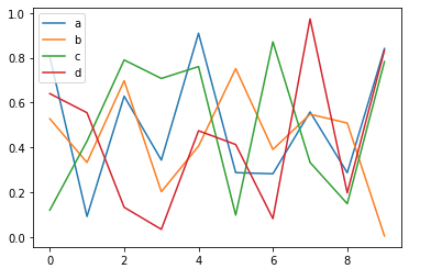
np.random.seed(999)
df = pd.DataFrame(np.random.rand(10, 4), columns=['a', 'b', 'c', 'd'])
我们直接调用plot方法进行展示。 这里有两个需要注意的地方:
- 该plot方法是通过Pandas调用的plot方法,而非matplotlib。
- 我们知道Python语言是无需分号进行结束语句的。此处的分号表示执行绘图渲染后直接显示图像。
df.plot();
![]()
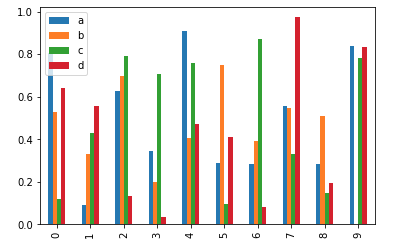
df.plot.bar();
![]()
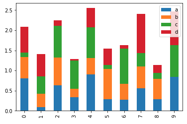
df.plot.bar(stacked=True);
![]()
四、更多
我们下篇将讲解matplotlib的相关知识点,欢迎关注机器学习前置教程系列,或我的个人博客http://blog.caiyongji.com/同步更新。