您现在的位置是：首页 > 文章详情

小白也能看懂的 AUC 详解

日期：2023-11-01点击：349收藏

简介

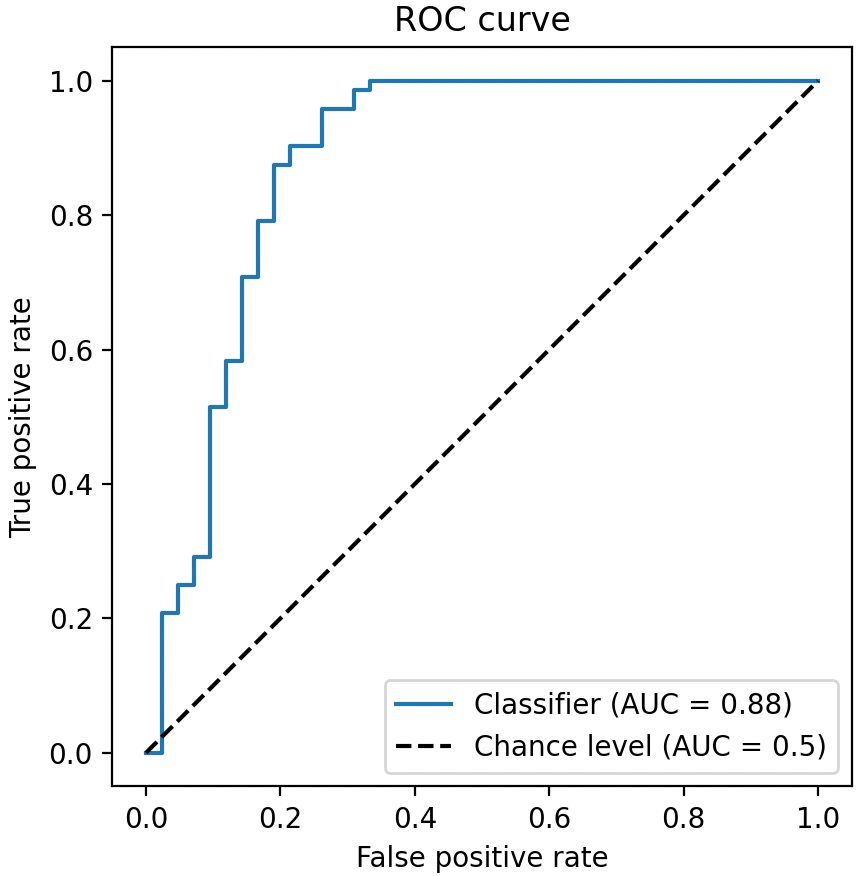
上篇文章小白也能看懂的 ROC 曲线详解介绍了 ROC 曲线。本文介绍 AUC。AUC 的全名为Area Under the ROC Curve，即 ROC 曲线下的面积，最大为 1。

根据 ROC 和 AUC 的关系，我们可以得到如下结论

ROC 曲线接近左上角 ---> AUC 接近 1：模型预测准确率很高
ROC 曲线略高于基准线 ---> AUC 略大于 0.5：模型预测准确率一般
ROC 低于基准线 ---> AUC 小于 0.5：模型未达到最低标准，无法使用

二分类 AUC

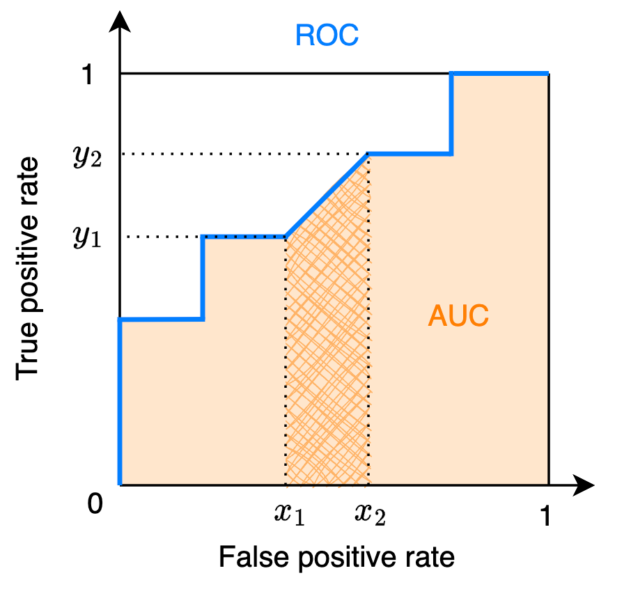
由 AUC 名称可知，可以先计算 ROC 曲线，得到 TPR 和 FPR 的坐标后再分段计算面积即可得到 AUC

下面是对应的 Python 代码

 def auc_from_roc(fpr, tpr): """ 计算ROC面积 fpr: 从小到大排序的fpr坐标 tpr: 从小到大排序的tpr坐标 """ area = 0 for i in range(len(fpr) - 1): area += trapezoid_area(fpr[i], fpr[i + 1], tpr[i], tpr[i + 1]) return area def trapezoid_area(x1, x2, y1, y2): """ 计算梯形面积 x1, x2: 横坐标 (x1 <= x2) y1, y2: 纵坐标 (y1 <= y2) """ base = x2 - x1 height_avg = (y1 + y2) / 2 return base * height_avg

也可以直接从真实标签和模型预测分数中计算 ROC，算法的时间复杂度为\(O(n\log n)\)，参考文献 1 中的算法 2

 # import numpy as np def auc_binary(y_true, y_score, pos_label): """ y_true：真实标签 y_score：模型预测分数 pos_label：正样本标签，如“1” """ num_positive_examples = (y_true == pos_label).sum() num_negtive_examples = len(y_true) - num_positive_examples tp, fp, tp_prev, fp_prev, area = 0, 0, 0, 0, 0 score = -np.inf for i in np.flip(np.argsort(y_score)): if y_score[i] != score: area += trapezoid_area(fp_prev, fp, tp_prev, tp) score = y_score[i] fp_prev = fp tp_prev = tp if y_true[i] == pos_label: tp += 1 else: fp += 1 area += trapezoid_area(fp_prev, fp, tp_prev, tp) area /= num_positive_examples * num_negtive_examples return area

多分类 AUC

现在考虑多分类的情况，假设类别数为\(C\)。

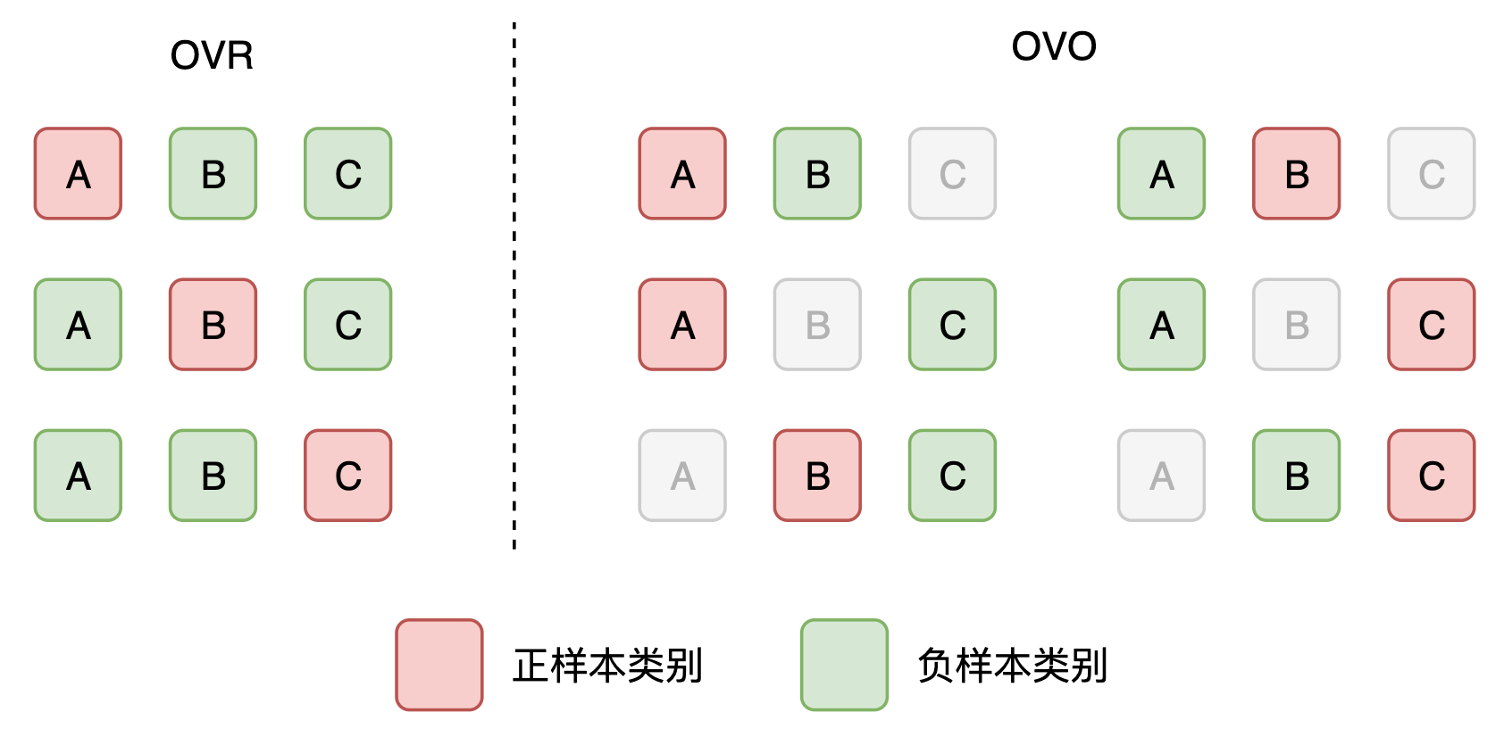
一种想法是将某一类别设为正样本类别，其余类别设为负样本类别，然后计算二分类下的 AUC。这种方法叫做一对多，即 One-Vs-Rest (OVR)。可以得到\(C\)个二分类的 AUC，然后计算平均数得到多分类的 AUC。

另一种想法是将某一类别设为正样本类别，另外一个类别（非自身）设为负样本类别计算二分类的 AUC。这种方法叫做一对一，即 One-Vs-One (OVO)。可以得到\(C(C-1)\)个二分类的 AUC，然后计算平均数。

当计算平均数时，可以考虑算数平均数（称为 macro），或者加权平均数（称为 weighted）。其中，加权为各类别的样本所占比例。因此，两两组合可以的得到四种计算多分类 AUC 的方法。值得一提的是，知名机器学习库 scikit-learn 的 roc_auc_score 函数包含了上述四种方法。

一对多 + 算数平均数（OVR + macro）
一对多 + 加权平均数（OVR + weighted）
一对一 + 算数平均数（OVO + macro）
一对一 + 加权平均数（OVO + weighted）

一对多 + 算数平均数

多分类 AUC 的计算公式为

\(\text{AUC}_\text{total}=\frac{1}{C}\sum_{c_i\in C}\text{AUC}(c_i)\)

其中\(\text{AUC}(c_i)\)是将类别\(c_i\)作为正样本类别（剩余作为负样本类别），计算的二分类 AUC。

 # sklearn.metrics.roc_auc_score(y_true, y_score, average='macro', multi_class='ovr') def auc_ovr_macro(y_true, y_score): auc = 0 C = max(y_true) + 1 for i in range(C): auc += auc_binary(y_true, y_score[:, i], pos_label=i) return auc / C

一对多 + 加权平均数

多分类 AUC 的计算公式为

\(\text{AUC}_\text{total}=\sum_{c_i\in C}\text{AUC}(c_i)p(c_i)\)

其中，权重\(p(c_i)=\frac{\sum\mathbb{I}\{y=c_i\}}{n}\)，即标签为\(c_i\)的样本所占比例，权重之和为 1。

 # sklearn.metrics.roc_auc_score(y_true, y_score, average='weighted', multi_class='ovr') def auc_ovr_weighted(y_true, y_score): auc = 0 C = max(y_true) + 1 n = len(y_true) for i in range(C): p = sum(y_true == i) / n auc += auc_binary(y_true, y_score[:, i], pos_label=i) * p return auc

一对一 + 算数平均数

多分类 AUC 的计算公式为

\(\text{AUC}_\text{total}=\frac{2}{C(C-1)}\sum_{{c_i,c_j}\in C,\ c_i<c_j}\text{AUC}(c_i,c_j)\)

其中，\(\text{AUC}(c_i,c_j)=\frac{\text{AUC}(c_i｜c_j)+\text{AUC}(c_j｜c_i )}{2}\)。即将\(c_i\)作为正样本类别、\(c_j\)作为负样本类别计算二分类 \(\text{AUC}(c_i｜c_j)\)；然后将\(c_j\)作为正样本类别、\(c_i\)作为负样本类别计算二分类 \(\text{AUC}(c_j｜c_i)\)。\(\text{AUC}(c_i,c_j)\) 为其计算的算数平均值。由于将\(c_i\)和\(c_j\)组合计算，共得到 \(C(C-1)/2\) 个二分类 AUC。

 # sklearn.metrics.roc_auc_score(y_true, y_score, average='macro', multi_class='ovo') def auc_ovo_macro(y_true, y_score): auc = 0 C = max(y_true) + 1 for i in range(C - 1): i_index = np.where(y_true == i)[0] for j in range(i + 1, C): j_index = np.where(y_true == j)[0] index = np.concatenate((i_index, j_index)) auc_i_j = auc_binary(y_true[index], y_score[index, i], pos_label=i) auc_j_i = auc_binary(y_true[index], y_score[index, j], pos_label=j) auc += (auc_i_j + auc_j_i) / 2 return auc * 2 / (C * (C - 1))

一对一 + 加权平均数

多分类 AUC 的计算公式为

\(\text{AUC}_\text{total}=\sum_{{c_i,c_j}\in C,\ c_i<c_j}\text{AUC}(c_i,c_j)p(c_i,c_j)\)

其中，权重\(p(c_i,c_j)=\frac{\sum\mathbb{I}\{y=c_i\}+\sum\mathbb{I}\{y=c_j\}}{(C-1)n}\)，即标签为\(c_i\)和\(c_j\)的样本所占比例，分母中的系数 \(C-1\) 使得权重之和为 1。

 # sklearn.metrics.roc_auc_score(y_true, y_score, average='weighted', multi_class='ovo') def auc_ovo_weighted(y_true, y_score): auc = 0 C = max(y_true) + 1 n = len(y_true) for i in range(C - 1): i_index = np.where(y_true == i)[0] for j in range(i + 1, C): j_index = np.where(y_true == j)[0] index = np.concatenate((i_index, j_index)) p = len(index) / n / (C - 1) auc_i_j = auc_binary(y_true[index], y_score[index, i], pos_label=i) auc_j_i = auc_binary(y_true[index], y_score[index, j], pos_label=j) auc += (auc_i_j + auc_j_i) / 2 * p return auc