继上一片的内容，这片来·讲一下sklearn来进行简单的人脸识别，这里用的方法是pca和svm
先导入必要的包和数据集

import numpy as np
import matplotlib.pyplot as plt
from scipy import stats

from sklearn.decomposition import PCA
from sklearn.svm import SVC
from sklearn import datasets

lfw_people = datasets.fetch_lfw_people(min_faces_per_person=70, \
                                       resize=0.4)

sklearn的人脸数据集包含5千多个不同人的人脸，但有些人的人脸只包含一张，

n_samples, h, w = lfw_people.images.shape
print('height and width of images:', h, w)

# The images in X have been collapsed into a 1D array
# just like for the handwritten digits
X = lfw_people.data

# X.shape[0] tells you the number of images (faces);
# this is the same as n_samples ahove
# X.shape[1] gives the number of pixels for each image
# or, "features"

print('X.shape', X.shape)
n_features = X.shape[1]


# the label/target to predict is the id of the person -- y is an integer
y = lfw_people.target
# target_names are actually names
target_names = lfw_people.target_names
print('target_names.shape', target_names.shape)
print('target_names', target_names)

# n_classes gives the number of people 
# Different from the number of faces (n_samples)!!
n_classes = target_names.shape[0]

print("Total dataset size:")
print("n_samples (number of faces): {0}".format(n_samples))
# n_features = 1850, which is 50x37, the dimension of the images.
print("n_features (number of pixels): {0}".format(n_features))
print("n_classes (number of people): {0}".format(n_classes))

通过打印可以看到数据集人脸的尺寸为50x37，为7类共1288张人脸

pca = PCA(n_components=4,whiten = True)
X_proj = pca.fit_transform(X[:500])
print("eigen vector",pca.components_)
print("...")
print('eigen value', pca.explained_variance_[:2])
print(np.var(X_proj[:,0]))
print(np.var(X_proj[:,1]))

取500组数据将其降维为4个维度，并进行归一化处理
explained_variance_，它代表降维后的各主成分的方差值。方差值越大，则说明越是重要的主成分

from sklearn import svm
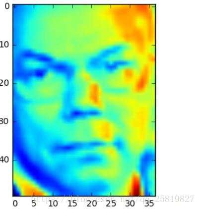
def plot_faces(n_features):
#     nside = 1
    X = lfw_people.data
#     fig, axes = plt.subplots(nside, nside, figsize=(8, 8))

    plt.imshow(X[5].reshape(50,37))
plot_faces(n_features= 16)
plt.show()

试着打一下其中的一幅图片

Xtrain = lfw_people.data[:1000]
Xtest = lfw_people.data[1000:,]
ytrain = lfw_people.target[:1000]
ytest = lfw_people.target[1000:,]
# Xtest = X[select_idx].reshape(1, -1)
# test_img = X[select_idx]
# ytest = y[select_idx]

# 
n_comp = 50

pca = PCA(n_comp, whiten = True)  

pca.fit(Xtrain)
# pca.fit(Xtest)

Xtrain_proj = pca.transform(Xtrain)
# projecting test data onto pca axes
Xtest_proj = pca.transform(Xtest)

print(Xtrain_proj.shape)
print(Xtest_proj.shape)


# ************************************* The SVM Section ********************************

# instantiating an SVM classifier
clf = svm.SVC(gamma=0.001, C=100.)

# apply SVM to training data and draw boundaries.
clf.fit(Xtrain_proj, ytrain)
# Use SVM-determined boundaries to make
# a prediction for the test data point.
ypred = clf.predict(Xtest_proj)

correct = np.sum(ytest == ypred)
print(correct/288*100)

接下来之前载入的数据用pca和svm进行训练识别，在1288个数据中取前1000组为训练集，后288个为测试集，pca将维为50维，并用训练集训练的模型对测试集进行预测，最后的测试精度为：81.25%,相对于现状流行的深度学习来说精度还是差了一点。