LazyLLM教程 | 第12讲：实践：用缓存、异步与向量引擎加速你的RAG

代码运行结果：

 

query: a, linear time: 9.894371032714844e-05, linear res: a
query: a, trie time: 7.939338684082031e-05, trie res: a
query: lazyllm, linear time: 0.04016876220703125, linear res: lazyllm
query: lazyllm, trie time: 0.00011754035949707031, trie res: lazyllm
query: zwitterionic, linear time: 0.08771300315856934, linear res: zwitterionic
query: zwitterionic, trie time: 0.00011014938354492188, trie res: zwitterionic

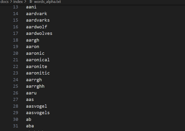
可以看到字典树与线性搜索均成功搜索对应的节点，但所用时间有着较为明显的差别：

线性搜索随着检索单词在词表中越往后，其耗时越来越久，而字典树的检索时间较为稳定。在37w词表中的最后一个单词检索过程中，线性搜索耗时0.0877s，字典树仅耗时0.0001s，时间节省了99.89%！因此，合理设计索引能够大大提升系统的检索效率。

2.结合场景，自己编写HNSW索引

在RAG场景中，往往建立高性能的ANN向量索引，以加速向量检索。根据上节课的介绍，相比大家对HNSW有了一定的了解，接下来我们按照上面构建索引的思路，同样构建一个HNSW索引，并对比LazyLLM内置的cosine相似度+默认索引情况下向量检索的速度。

 

HNSW索引的实现依赖hnswlib库，热门的向量数据库Milvus底层的ANN库之一就是hnswlib, 为milvus提供HNSW检索。具体代码如下（GitHub链接：

https://github.com/LazyAGI/Tutorial/blob/282ffb74e3fe7c5c28df4ad498ed972973dfbc62/rag/codes/chapter12/retriever_with_custom_index_hnsw.py#L19）：

class HNSWIndex(IndexBase):
    def __init__(
            self,
            embed: Dict[str, Callable],
            store: StoreBase,
            max_elements: int = 10000, # 定义索引最大容量
            ef_construction: int = 200,    # 平衡索引构建速度和搜索准确率，越大准确率越高但是构建速度越慢
            M: int = 16,    # 表示在建表期间每个向量的边数目量，M越高，内存占用越大，准确率越高，同时构建速度越慢
            dim: int = 1024, # 向量维度
            **kwargs
        ):
        self.embed = embed
        self.store = store
        # 由于hnswlib中的向量id不能为str，故建立label用于维护向量编号
        # 创建字典以维护节点id和hnsw中向量id的关系
        self.uid_to_label = {}
        self.label_to_uid = {}
        self.next_label = 0
        #初始化hnsw_index
        self._index_init(max_elements, ef_construction, M, dim)

    def _index_init(self, max_elements, ef_construction, M, dim):
        # hnswlib支持多种距离算法：l2、IP内积和cosine
        self.index = hnswlib.Index(space='cosine', dim=dim)
        self.index.init_index(
            max_elements=max_elements,
            ef_construction=ef_construction,
            M=M,
            allow_replace_deleted=True
        )
        self.index.set_ef(100) # 设置搜索时的最大近邻数量，较高值会导致更好的准确率，但搜索速度会变慢
        self.index.set_num_threads(8) # 设置在批量搜索和构建索引过程中使用的线程数

    @override
    def update(self, nodes: List['DocNode']):
        if not nodes or nodes[0]._group != 'block':
            return
        # 节点向量化，这里仅展示使用默认的embedding model
        parallel_do_embedding(self.embed, [], nodes=nodes, group_embed_keys={'block': ["__default__"]})
        vecs = []    # 向量列表
        labels = []    # 向量id列表
        for node in nodes:
            uid = str(node._uid)
            # 记录uid和label的关系，若为新的uid，则写入next_label
            if uid in self.uid_to_label:
                label = self.uid_to_label[uid]
            else:
                label = self.next_label
                self.uid_to_label[uid] = label
                self.next_label += 1
            # 取默认embedding结果
            vec = node.embedding['__default__'] 
            vecs.append(vec)
            labels.append(label)
            self.label_to_uid[label] = uid
        
        # 根据向量建立hnsw索引
        data = np.vstack(vecs)
        ids  = np.array(labels, dtype=int)
        self.index.add_items(data, ids)

    @override
    def remove(self, uids, group_name=None):
        """
        标记删除一批 uid 对应的向量，并清理映射
        """
        if group_name != 'block':
            return
        for uid in map(str, uids):
            if uid not in self.uid_to_label:
                continue
            label = self.uid_to_label.pop(uid)
            self.index.mark_deleted(label)
            self.label_to_uid.pop(label, None)

    @override
    def query(
        self,
        query: str,
        topk: int,
        embed_keys: List[str],
        **kwargs,
    ) -> List['DocNode']:
        # 生成查询向量
        parts = [self.embed[k](query) for k in embed_keys]
        qvec = np.concatenate(parts)
        # 调用hnsw knn_query方法进行向量检索
        labels, distances = self.index.knn_query(qvec, k=topk, num_threads=self.index.num_threads)
        results = []
        #取检索topk
        for lab, dist in zip(labels[0], distances[0]):
            uid = self.label_to_uid.get(lab)
            results.append(uid)
            if len(results) >= topk:
                break
        # 从store获取对应uid的节点
        return self.store.get_nodes(group_name='block', uids=results) if len(results) > 0 else []


def test_hnsw_index():
    dataset_path = os.path.join(DOC_PATH, "test")
    docs1 = lazyllm.Document(dataset_path=dataset_path, embed=embedding_model)
    docs1.create_node_group(name='block', transform=(lambda d: d.split('\n')))
    docs1.register_index("hnsw", HNSWIndex, docs1.get_embed(), docs1.get_store())
    retriever1 = lazyllm.Retriever(docs1, group_name="block", similarity="cosine", topk=3)
    retriever2 = lazyllm.Retriever(docs1, group_name="block", index="hnsw", topk=3)
    retriever1.start()
    retriever2.start()
    q = "证券监管？"
    st = time.time()
    res = retriever1(q)
    et = time.time()
    context_str = "\n---------\n".join([r.text for r in res])
    LOG.info(f"query: {q}, default time: {et - st}, default res:\n {context_str}")

    st = time.time()
    res = retriever2(q)
    et = time.time()
    context_str = "\n---------\n".join([r.text for r in res])
    LOG.info(f"query: {q}, HNSW time: {et - st}, HNSW res: \n{context_str}")

test_hnsw_index()

运行结果如下所示：

query: 证券监管？, default time: 0.5182957649230957, default res:
 金融监管部门的保护措施
---------
为规范证券公司资金账户管理工作，防范业务风险，保护客户合法权益，根据《中
---------
 为贯彻落实《证券经纪业务管理办法》 ，引导证券公司规范开展证券经纪业务，协
query: 证券监管？, HNSW time: 0.021764516830444336, HNSW res: 
金融监管部门的保护措施
---------
 为贯彻落实《证券经纪业务管理办法》 ，引导证券公司规范开展证券经纪业务，协
---------
为规范证券公司资金账户管理工作，防范业务风险，保护客户合法权益，根据《中

可以看到，使用默认的cosine相似度和默认索引进行向量检索用时0.518s，而使用自己实现的HNSW索引执行向量检索耗时0.022s，时间节省约95%。这个结论和标量索引实践一致，即通过建立高效索引，“以空间换时间”，可以大大降低计算量，提高检索效率。

 

实践三.从零开始，使用高性能向量数据库Milvus

向量索引很强大，但是从0开始手搓一个高性能索引成本比较高。细心的你一定发现了——在先前的存储配置中，Milvus向量数据库的配置参数中已经包含了索引相关的配置，没错！向量数据库早已把这些高性能的向量索引，实际研发过程中，我们只需要使用这些高性能的向量数据库，便可实现高性能的向量检索！

 

1.原生Milvus使用方式简介

安装

在本次实践中，我们使用 Milvus Lite，它是pymilvus 中包含的一个 python 库，可以嵌入到应用程序中。Milvus 还支持在Docker和Kubernetes上部署，适用于生产用例。运行下方命令即可完成pymilvus的安装。

pip install -U pymilvus

使用

首先我们使用以下代码创建一个milvus客户端。

from pymilvus import MilvusClient
# 创建milvus客户端，传入本地数据库的存储路径，若路径不存在则创建
client = MilvusClient("dbs/origin_milvus.db")

在 Milvus 中，我们需要一个 Collections 来存储向量及其相关元数据。它相当于传统 SQL 数据库中的表格。创建 Collections 时，可以定义 Schema 和索引参数来配置向量规格，如维度（dimension）、索引类型（index_params）和距离度量（metric_type）等。

（代码GitHub链接：

https://github.com/LazyAGI/Tutorial/blob/a09a84cdf0585a5c9d52af6db0e965be95d03123/rag/codes/chapter12/use_original_milvus.py#L8）

# 初始化阶段，如果已存在同名collection，则先删除
if client.has_collection(collection_name="demo_collection"):
    client.drop_collection(collection_name="demo_collection")
client.create_collection(
    collection_name="demo_collection",
    dimension=1024,
)

🚨注意：create_collection支持更多的入参，如主键列名primary_field_name、向量列名vector_field_name、向量索引参数index_params、相似度参数metric_type等，此处仅介绍基本用法，其余均使用默认参数。

 

随后准备文档切片，进行向量化后按照milvus接受的格式创建数据集，并注入数据库中，这里我们额外增加了一个字段subject（学科），用于充当数据的metadata。

（代码GitHub链接：

https://github.com/LazyAGI/Tutorial/blob/a09a84cdf0585a5c9d52af6db0e965be95d03123/rag/codes/chapter12/use_original_milvus.py#L16）

docs = [
    "Artificial intelligence was founded as an academic discipline in 1956.",
    "Alan Turing was the first person to conduct substantial research in AI.",
    "Born in Maida Vale, London, Turing was raised in southern England.",
]
vecs =[embedding_model(doc) for doc in docs] 
data = [
    {"id": i, "vector": vecs[i], "text": docs[i], "subject": "history"}
    for i in range(len(vecs))
]
# 数据注入
res = client.insert(collection_name="demo_collection", data=data)
print(f"Inserted data into client:\n {res}")

进行query检索时，同样需要先将query进行向量化，随后在client中调用search方法，指定对应的collection以及检索数量，并且支持指定输出哪些字段（output_fields）。

（代码GitHub链接：

https://github.com/LazyAGI/Tutorial/blob/a09a84cdf0585a5c9d52af6db0e965be95d03123/rag/codes/chapter12/use_original_milvus.py#L30）

query = "Who is Alan Turing?"
# query向量化
q_vec = embedding_model(query)
# 检索
res = client.search(
    collection_name="demo_collection",    # 指定collection
    data=[q_vec],
    limit=2,    # 指定检索数量（top_k）
    output_fields=["text", "subject"],    #指定检索结果中包含的字段
)
print(f"Query: {query} \nSearch result:\n {res}")

milvus不仅支持简单高效的向量检索，同时支持使用元数据作为过滤字段，实现标量索引+向量索引的符合检索。下面的代码中，我们同样创建3个文段，并在数据注入是设置subject为不同的学科。在检索方法search的入参中，我们输入filter参数，以设置期望过滤的数据。

（代码GitHub链接：

https://github.com/LazyAGI/Tutorial/blob/a09a84cdf0585a5c9d52af6db0e965be95d03123/rag/codes/chapter12/use_original_milvus.py#L43）

docs = [
    "Machine learning has been used for drug design.",
    "Computational synthesis with AI algorithms predicts molecular properties.",
    "DDR1 is involved in cancers and fibrosis.",
]
vecs =[embedding_model(doc) for doc in docs]
data = [
    {"id": 3 + i, "vector": vecs[i], "text": docs[i], "subject": "biology"}
    for i in range(len(vecs))
]
client.insert(collection_name="demo_collection", data=data)
res = client.search(
    collection_name="demo_collection",
    data=[embedding_model("tell me AI related information")],
    filter="subject == 'biology'",    # 期望过滤的字段
    limit=2,
    output_fields=["text", "subject"],
)
print(f"Filter Query: {query} \nSearch result:\n {res}")

我们结合以上使用方式，结合LazyLLM的其他组建重新搭建一个简易的RAG系统

（代码GitHub链接：

https://github.com/LazyAGI/Tutorial/blob/282ffb74e3fe7c5c28df4ad498ed972973dfbc62/rag/codes/chapter12/rag_with_original_milvus.py#L1）：

import os

import lazyllm
from lazyllm.tools.rag import SimpleDirectoryReader, SentenceSplitter
from lazyllm.tools.rag.doc_node import MetadataMode

from pymilvus import MilvusClient

from online_models import embedding_model, llm, rerank_model

DOC_PATH = os.path.abspath("docs")

###################### 文件入库 ###################################
# milvus client初始化
client = MilvusClient("dbs/rag_milvus.db")
if client.has_collection(collection_name="demo_collection"):
    client.drop_collection(collection_name="demo_collection")

client.create_collection(
    collection_name="demo_collection",
    dimension=1024,
)

# 加载本地文件，并解析 -- block切片 -- 向量化 -- 入库
dataset_path = os.path.join(DOC_PATH, "test")
docs = SimpleDirectoryReader(input_dir=dataset_path)()
block_transform = SentenceSplitter(chunk_size=256, chunk_overlap=25)

nodes = []
for doc in docs:
    nodes.extend(block_transform(doc))

# 切片向量化
vecs = [embedding_model(node.get_text(MetadataMode.EMBED)) for node in nodes]
data = [
    {"id": i, "vector": vecs[i], "text": nodes[i].text}
    for i in range(len(vecs))
]
#数据注入
res = client.insert(collection_name="demo_collection", data=data)

###################### 检索问答 ###################################
query = "证券管理的基本规范？"

# 检索与生成
prompt = '你是一个友好的 AI 问答助手，你需要根据给定的上下文和问题提供答案。\
        根据以下资料回答问题：\
        {context_str} \n '
llm.prompt(lazyllm.ChatPrompter(instruction=prompt, extro_keys=['context_str']))

q_vec = embedding_model(query)
res = client.search(
    collection_name="demo_collection",
    data=[q_vec],
    limit=12,
    output_fields=["text"],
)

# 提取检索结果
contexts = [res[0][i].get('entity').get("text", "") for i in range(len(res[0]))]

# 重排
rerank_res = rerank_model(text=query, documents=contexts, top_n=3)
rerank_contexts = [contexts[res[0]] for res in rerank_res]

context_str = "\n-------------------\n".join(rerank_contexts)

res = llm({"query": query, "context_str": context_str})
print(res)

在上述代码中，我们首先使用原生的使用方式定义了milvus client，随后使用LazyLLM自带的文档解析器提取文档内容，并转换为切片，向量化后注入向量数据库中。随后进行query检索，提取检索内容并执行重排序后，给到大模型进行回答。

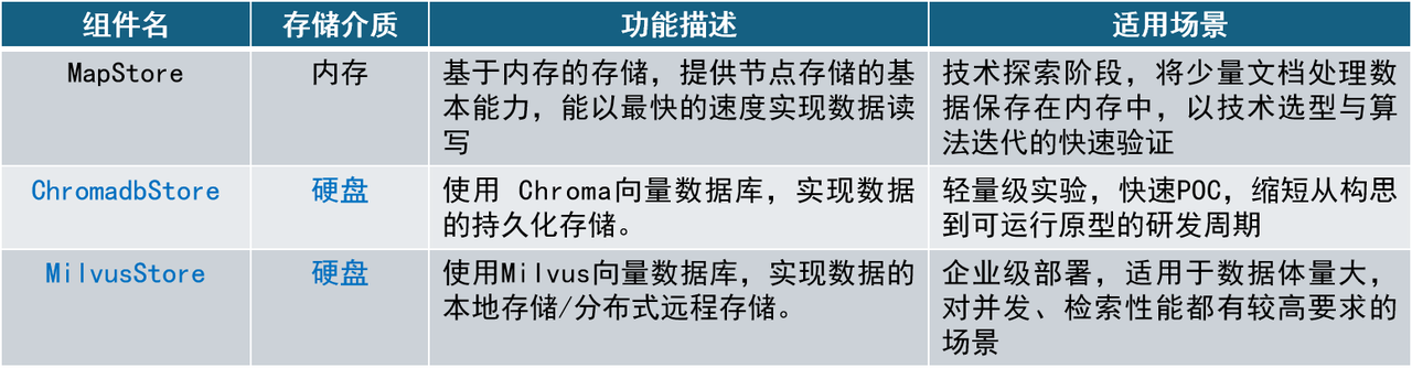
2.在LazyLLM中使用Milvus

从上述的实践内容中我们不难发现，milvus可以实现持久化存储、检索性能强。但是原生milvus的使用方式确实有些复杂，用户需要花较大的成本从头学习如何使用一个向量数据库。这对于开发者来说多少有些“折腾”。索性LazyLLM已经将Milvus完美适配，按照先前介绍的，只需要进行简单的存储及索引后端配置，便可轻松将milvus接入到RAG系统当中。具体配置方法是需要在上述存储后端配置store_conf中额外添加字段 'indices' ，indices是一个python字典，key 是索引类型名称，value 是该索引类型所需要的参数，具体配置如下：

store_conf = {
    'type': 'map',
    'indices': {
        'smart_embedding_index': {
            'backend': 'milvus',                        # 设定索引使用Milvus后端
              'kwargs': {
                'uri': 'dbs/test.db',               # Milvus数据存储地址
                  'index_kwargs': {        
                    'index_type': 'HNSW',                # 设置索引类型
                    'metric_type': 'COSINE',       # 设置度量类型
                }
            },
        },
    },
}

• key: 'smart_embedding_index'（使用milvus向量数据库内置向量索引，以实现高效向量检索）

• values:

  ⚒️'backend': 索引后端，当前仅支持传入'milvus'，已使用Milvus向量数据库。

  ⚒️'kwargs'：选择对应索引后端时，额外的配置项，选择milvus时，配置项与存储后端使用milvus一致，均为uri和index_kwargs。

 

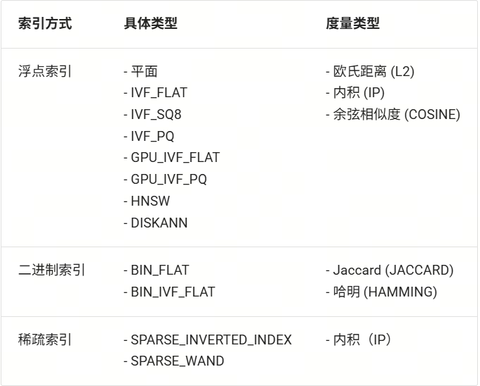
Milvus 支持多种索引方式，一般来说浮点索引（即对稠密向量进行索引）的使用场景较多，适用于大规模数据的语义检索，二进制索引和稀疏索引适用于数据集较小的情况，可以保证较高的召回率。每种索引方式都有对应的推荐度量方式，您可以根据需求按照下表进行选择：

 

我们根据以上milvus配置，使用LazyLLM内置的SmartEmbeddingIndex实现Milvus的索引接入，并同样与使用默认索引的Retriever比较检索速度

（完整代码见Github链接：

https://github.com/LazyAGI/Tutorial/blob/patch-1/rag/codes/chapter12/retriever_with_custom_index_hnsw.py#L118）：

import os
import time

import lazyllm
from lazyllm import LOG

from online_models import embedding_model

DOC_PATH = os.path.abspath("docs")

milvus_store_conf = {
    'type': 'map',
    'indices': {
        'smart_embedding_index': {
            'backend': 'milvus',
            'kwargs': {
                'uri': "dbs/test_map_milvus.db",
                'index_kwargs': {
                    'index_type': 'HNSW',
                    'metric_type': 'COSINE',
                }
            },
        },
    },
}
dataset_path = os.path.join(DOC_PATH, "test")

docs = lazyllm.Document(dataset_path=dataset_path, embed=embedding_model, store_conf=milvus_store_conf)

# 使用默认索引
retriever1 = lazyllm.Retriever(docs, group_name="MediumChunk", topk=6, similarity="cosine")
# 使用milvus内置HNSW索引
retriever2 = lazyllm.Retriever(docs, group_name="MediumChunk", topk=6, index='smart_embedding_index')
retriever1.start()
retriever2.start()

q = "证券监管？"
st = time.time()
res = retriever1(q)
et = time.time()
LOG.info(f"query: {q}, default time: {et - st}")

st = time.time()
res = retriever2(q)
et = time.time()
LOG.info(f"query: {q}, milvus time: {et - st}")

在store_conf的配置中，存储后端和索引后端是独立的两部分，但是如果存储类型选择milvus的情况下，由于kwargs中已经包含了索引配置信息，因此无需额外配置indices，即可实现内置的向量检索。

可以看到，使用 Milvus 时，和将 Milvus 用作存储后端一致，将索引配置indices传入 store_conf ，然后在 Retriever 中指定 index='smart_embedding_index' 即可。相比于原生的使用方式，使用store_conf使向量数据库的使用更加简单，代码也更加简洁可读。程序运行的结果如下：

query: 证券监管？, default time: 0.16447973251342773
query: 证券监管？, milvus time: 0.02178812026977539

使用LazyLLM内置的Milvus执行检索相比默认的向量索引，检索时间节省约86.75%。使用 Milvus 作为索引后端，基于多 embedding 召回策略构建 RAG 系统代码如下所示，下方代码展示了同时使用稠密和稀疏检索的方式：

import lazyllm
from lazyllm import bind, deploy

milvus_store_conf = {
    'type': 'milvus',
    'kwargs': {
        'uri': "milvus.db",
        'index_kwargs': [
            {
                'embed_key': 'bge_m3_dense',
                'index_type': 'IVF_FLAT',
                'metric_type': 'COSINE',
            },
            {
                'embed_key': 'bge_m3_sparse',
                'index_type': 'SPARSE_INVERTED_INDEX',
                'metric_type': 'IP',
            }
        ]
    },
}

bge_m3_dense = lazyllm.TrainableModule('bge-m3')
bge_m3_sparse = lazyllm.TrainableModule('bge-m3').deploy_method((deploy.AutoDeploy, {'embed_type': 'sparse'}))
embeds = {'bge_m3_dense': bge_m3_dense, 'bge_m3_sparse': bge_m3_sparse}
document = lazyllm.Document(dataset_path='/path/to/your/document',
           embed=embeds,
           store_conf=milvus_store_conf)

document.create_node_group(name="block", transform=lambda s: s.split("\n") if s else '')
bge_rerank = lazyllm.TrainableModule("bge-reranker-large")

with lazyllm.pipeline() as ppl:
    with lazyllm.parallel().sum as ppl.prl:
        ppl.prl.retriever1 = lazyllm.Retriever(doc=document,
                         group_name="block",
                         embed_keys=['bge_m3_dense'],
                         topk=3)
        ppl.prl.retriever = lazyllm.Retriever(doc=document,
                         group_name="block",
                         embed_keys=['bge_m3_sparse'],
                         topk=3)
    ppl.reranker = lazyllm.Reranker(name='ModuleReranker',model=bge_rerank, topk=3) | bind(query=ppl.input)
    ppl.formatter = (
      lambda nodes, query: dict(
          context_str=[node.get_content() for node in nodes],
          query=query)
    ) | bind(query=ppl.input)
    
    ppl.llm = lazyllm.OnlineChatModule().prompt(lazyllm.ChatPrompter(instruction=prompt, extra_keys=['context_str']))
webpage = lazyllm.WebModule(ppl, port=23492).start().wait()

结合之前介绍的存储配置，我们将第七讲中的RAG系统进行存储和索引的全面优化，全面提升系统的执行效率，代码如下

（GitHub链接：

https://github.com/LazyAGI/Tutorial/blob/patch-4/rag/codes/chapter12/rag_use_milvus_store.py）：

import os

import lazyllm
from lazyllm import Reranker

from online_models import embedding_model, llm, rerank_model    # 使用线上模型

DOC_PATH = os.path.abspath("docs")

# milvus存储和索引配置
milvus_store_conf = {
    'type': 'milvus',
    'kwargs': {
        'uri': "dbs/milvus1.db",
        'index_kwargs': {
        'index_type': 'HNSW',
        'metric_type': 'COSINE',
        }
    }
}
dataset_path = os.path.join(DOC_PATH, "test")

# 定义Document，传入配置以使用milvus存储及检索
docs = lazyllm.Document(dataset_path=dataset_path, embed=embedding_model, store_conf=milvus_store_conf)
#创建句子节点组
docs.create_node_group(name='sentence', parent="MediumChunk", transform=(lambda d: d.split('。')))
#创建MediumChunk、sentence节点组多路召回，
retriever1 = lazyllm.Retriever(docs, group_name="MediumChunk", topk=6, index='smart_embedding_index')
retriever2 = lazyllm.Retriever(docs, group_name="sentence", target="MediumChunk", topk=6, index='smart_embedding_index')
retriever1.start()
retriever2.start()
#创建reranker
reranker = Reranker('ModuleReranker', model=rerank_model, topk=3)

prompt = '你是一个友好的 AI 问答助手，你需要根据给定的上下文和问题提供答案。\
        根据以下资料回答问题：\
        {context_str} \n '
llm.prompt(lazyllm.ChatPrompter(instruction=prompt, extro_keys=['context_str']))

query = "证券管理有哪些准则？"

nodes1 = retriever1(query=query)
nodes2 = retriever2(query=query)
rerank_nodes = reranker(nodes1 + nodes2, query)
context_str = "\n======\n".join([node.get_content() for node in rerank_nodes])
print(f"context_str: \n{context_str}")
res = llm({"query": query, "context_str": context_str})
print(res)

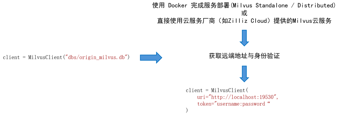
Milvus不仅支持本地db文件链接，同时支持远程服务器端点的接入。

 

例如，我们期望在Linux系统上部署Milvus Standalone服务。

• 安装Docker，并根据 Milvus 官方文档检查硬件与软件要求。

• 在Docker中安装Milvus，安装脚本：

# 下载安装脚本
curl -sfL https://raw.githubusercontent.com/milvus-io/milvus/master/scripts/standalone_embed.sh -o standalone_embed.sh

# 启动Docker容器
bash standalone_embed.sh start

• 安装结果：

  ⚒️名为 Milvus 的 docker 容器在19530端口启动。要更改 Milvus 的默认配置，需将设置添加到当前文件夹中的user.yaml文件，然后重新启动服务。

  ⚒️Milvus 数据卷被映射到当前文件夹中的volumes/milvus。

实践四.工程优化技巧，缓存与并行检索

在先前的第11讲中我们提到了一些工程优化技巧，例如缓存机制、多任务并行等。接下来我们分别进行实践。

1.使用K-V缓存

本次实践使用简单的k-v dict模拟缓存机制，我们搭建一个从RAG系统启动至检索的过程，并设置kv字典用于保存检索过的query与节点集合，并测试有无缓存机制时系统的检索时间：

milvus_store_conf = {
    'type': 'map',
    'indices': {
        'smart_embedding_index': {
        'backend': 'milvus',
        'kwargs': {
            'uri': "dbs/test_cache.db",
            'index_kwargs': {
                'index_type': 'HNSW',
                'metric_type': 'COSINE',
            }
        },
        },
    },
}
dataset_path = os.path.join(DOC_PATH, "test")

docs = lazyllm.Document(
    dataset_path=dataset_path,
    embed=embedding_model,
    store_conf=milvus_store_conf
)
docs.create_node_group(name='sentence', parent="MediumChunk", transform=(lambda d: d.split('。')))

retriever1 = lazyllm.Retriever(docs, group_name="MediumChunk", topk=6, index='smart_embedding_index')
retriever2 = lazyllm.Retriever(docs, group_name="sentence", target="MediumChunk", topk=6, index='smart_embedding_index')
retriever1.start()
retriever2.start()

reranker = Reranker('ModuleReranker', model=rerank_model, topk=3)

# 设置固定query
query = "证券管理的基本规范？"

# 运行5次没有缓存机制的检索流程，并记录时间
time_no_cache = []
for i in range(5):
    st = time.time()
    nodes1 = retriever1(query=query)
    nodes2 = retriever2(query=query)
    rerank_nodes = reranker(nodes1 + nodes2, query)
    et = time.time()
    t = et - st
    time_no_cache.append(t)
    print(f"No cache 第 {i+1} 次查询耗时：{t}s")

# 定义dict[list]，存储已检索的query和节点集合，实现简易的缓存机制
kv_cache = defaultdict(list)
for i in range(5):
    st = time.time()
    #如果query未在缓存中，则执行正常的检索流程，若query命中缓存，则直接取缓存中的节点集合
    if query not in kv_cache:
        nodes1 = retriever1(query=query)
        nodes2 = retriever2(query=query)
        rerank_nodes = reranker(nodes1 + nodes2, query)
        # 检索完毕后，缓存query及检索节点
        kv_cache[query] = rerank_nodes
    else:
        rerank_nodes = kv_cache[query]
    et = time.time()
    t = et - st
    time_no_cache.append(t)
    print(f"KV cache 第 {i+1} 次查询耗时：{t}s")

以上代码中主要实现了RAG系统中的启动和检索环节，对于检索环节，使用字典的形式实现了kv cache机制，检索开始时首先会检查当前查询的节点是否已经在缓存当中，如果存在，即为缓存命中，直接取缓存中的查询结果即可，反之则进行正常的检索流程，并在最后将检索结果存入缓存当中。程序运行后得到如下输出：

No cache 第 1 次查询耗时：1.3868563175201416s
No cache 第 2 次查询耗时：1.277320146560669s
No cache 第 3 次查询耗时：1.2744269371032715s
No cache 第 4 次查询耗时：1.3921117782592773s
No cache 第 5 次查询耗时：1.3207831382751465s
KV cache 第 1 次查询耗时：1.4092140197753906s
KV cache 第 2 次查询耗时：2.384185791015625e-07s
KV cache 第 3 次查询耗时：1.430511474609375e-06s
KV cache 第 4 次查询耗时：2.384185791015625e-07s
KV cache 第 5 次查询耗时：2.384185791015625e-07s

可以看到，当系统没有缓存查询结果时，每次查询的时间均在1点几秒，而使用缓存的情况下，除了第一次正常检索，其余检索均在瞬间完成，因此，合理设计缓存机制能够在高效的向量索引基础之上进一步提升系统检索性能。

 

🚨注意：实践的目的主要是为了展示缓存机制对于检索性能的提升，实际生产过程当中，通常会使用内存数据管理系统（如Redis）实现相关功能。同时，需要考虑多种因素以建立完善的缓存机制。如：

 

• 文档更新是缓存清理

• 高热query的具体定义

• 相似query命中

• ...

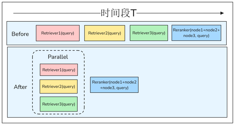
2.并行执行，多路召回效率提升

您可以发现，先前多路召回的场景中，检索器依次执行检索，这种流程其实是很低效的。考虑到检索器之间不存在耦合，因此，我们可以使用LazyLLM的Flow组件中的parallel实现检索器的并行多路召回。

 

代码如下：

milvus_store_conf = {
    'type': 'milvus',
    'kwargs': {
        'uri': "dbs/test_parallel.db",
        'index_kwargs': {
        'index_type': 'HNSW',
        'metric_type': 'COSINE',
        }
    }
}
dataset_path = os.path.join(DOC_PATH, "test")

docs1 = lazyllm.Document(
    dataset_path=dataset_path,
    embed=embedding_model,
    store_conf=milvus_store_conf
)
docs1.create_node_group(name='sentence', parent="MediumChunk", transform=(lambda d: d.split('。')))
retriever1 = lazyllm.Retriever(docs1, group_name="MediumChunk", topk=3)
retriever2 = lazyllm.Retriever(docs1, group_name="sentence", target="MediumChunk", topk=3)

retriever1.start()
retriever2.start()

with lazyllm.parallel().sum as prl:
    prl.r1 = retriever1
    prl.r2 = retriever2

query = "证券管理的基本规范？"

st = time.time()
retriever1(query=query)
retriever2(query=query)
et1 = time.time()
prl(query)
et2 = time.time()
print(f"顺序检索耗时：{et1-st}s")
print(f"并行检索耗时：{et2-et1}s")

执行以上代码获得输出：

顺序检索耗时：0.0436248779296875s
并行检索耗时：0.025980472564697266s

可以看出，使用并行检索可以有效节省检索时间，提升检索效率。最后，我们综合以上所有优化策略实现一个优化效率后的高性能RAG系统：

milvus_store_conf = {
    'type': 'milvus',
    'kwargs': {
        'uri': "dbs/test_rag.db",
        'index_kwargs': {
        'index_type': 'HNSW',
        'metric_type': 'COSINE',
        }
    }
}
dataset_path = os.path.join(DOC_PATH, "test")
# 定义kv缓存
kv_cache = defaultdict(list)

docs1 = lazyllm.Document(dataset_path=dataset_path, embed=embedding_model, store_conf=milvus_store_conf)
docs1.create_node_group(name='sentence', parent="MediumChunk", transform=(lambda d: d.split('。')))

prompt = '你是一个友好的 AI 问答助手，你需要根据给定的上下文和问题提供答案。\
    根据以下资料回答问题：\
    {context_str} \n '

with lazyllm.pipeline() as recall:
    # 并行多路召回
    with lazyllm.parallel().sum as recall.prl:
        recall.prl.r1 = lazyllm.Retriever(docs1, group_name="MediumChunk", topk=6)
        recall.prl.r2 = lazyllm.Retriever(docs1, group_name="sentence", target="MediumChunk", topk=6)
    recall.reranker = lazyllm.Reranker(name='ModuleReranker',model=rerank_model, topk=3) | lazyllm.bind(query=recall.input)
    recall.cache_save = (lambda nodes, query: (kv_cache.update({query: nodes}) or nodes)) | lazyllm.bind(query=recall.input)
    
with lazyllm.pipeline() as ppl:
    # 缓存检查
    ppl.cache_check = lazyllm.ifs(
        cond=(lambda query: query in kv_cache),
        tpath=(lambda query: kv_cache[query]),
        fpath=recall
    )
    ppl.formatter = (
        lambda nodes, query: dict(
            context_str="\n".join(node.get_content() for node in nodes),
            query=query)
    ) | lazyllm.bind(query=ppl.input)
    ppl.llm = llm.prompt(lazyllm.ChatPrompter(instruction=prompt, extro_keys=['context_str']))

w = lazyllm.WebModule(ppl, port=23492, stream=True).start().wait()

使用 vLLM 框架启动量化模型服务

vLLM 是一个专门为大语言模型（LLM）推理优化的高效推理框架，旨在大幅提升大模型的推理速度，并降低显存占用。它采用了一系列优化技术，如高效的连续批处理（PagedAttention）和动态 KV 缓存管理，使其在 GPU 推理场景下相比传统方法更具优势。

 

1.直接启动本地服务

LazyLLM 原生支持了 LightLLM、LMDeploy 和 vLLM 三种大模型推理加速框架和 Infinity 嵌入模型加速框架，用户在使用时仅需通过 TrainableModule.deploy_method 指定对应的框架即可。

from lazyllm import TrainableModule, deploy

llm = TrainableModule('model_name').deploy_method(deploy.vllm)

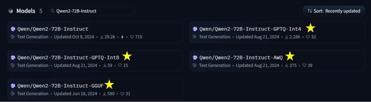
vLLM 支持多数大模型的推理服务，您可以先确认您想用的模型是否在 LazyLLM支持的模型列表中。在这个列表中后面带有 AWQ、4bit 等标识的都是量化模型，您可以根据您的需求选择一个量化模型然后启动对话服务，例如：

from lazyllm import TrainableModule, deploy

llm = TrainableModule('Qwen2-72B-Instruct-AWQ').deploy_method(deploy.vllm).start()
print(llm("hello, who are you?"))

我们以 Qwen2-72B-Instruct 和它的 AWQ 量化版本为例，对比一下二者的大小及运行速度。运行BF16或FP16 的 Qwen2-72B-Instruct 模型运行需要至少144GB显存（例如2xA100-80G或5xV100-32G）；运行 Int4 模型至少需要 48GB 显存（例如1xA100-80G或2xV100-32G），是原来的33%

（数据来源于 Qwen 官方魔塔社区：

https://modelscope.cn/models/qwen/Qwen-72B/）。

 

下面我们简单对比一下二者的运行速度，更严谨的情况下可以对比多次执行的差异

（完整代码见GitHub链接：

https://github.com/LazyAGI/Tutorial/blob/patch-4/rag/codes/chapter12/use_quantized_llm.py）：

import time
from lazyllm import TrainableModule, deploy, launchers

start_time = time.time()
llm = TrainableModule('Qwen2-72B-Instruct').deploy_method(
        deploy.Vllm).start()

end_time = time.time()
print("原始模型加载耗时：", end_time-start_time)

start_time = time.time()
llm_awq = TrainableModule('Qwen2-72B-Instruct-AWQ').deploy_method(deploy.Vllm).start()
end_time = time.time()
print("AWQ量化模型加载耗时：", end_time-start_time)

query = "生成一份1000字的人工智能发展相关报告"

start_time = time.time()
llm(query)
end_time = time.time()
print("原始模型耗时：", end_time-start_time)

start_time = time.time()
llm_awq(query)
end_time = time.time()
print("AWQ量化模型耗时：", end_time-start_time)

同样在 4 张 A800 卡加载和执行的速度如下所示：

 

• 原始模型加载耗时： 129.6051540374756

• 原始模型耗时： 13.104065895080566

• AWQ量化模型加载耗时： 86.4980857372284

• AWQ量化模型耗时： 8.81701111793518

 

LazyLLM 输出的日志信息中的 token/s 信息分别为：

 

• INFO 03-12 19:52:50 metrics.py:341] Avg prompt throughput: 6.6 tokens/s, Avg generation throughput: 30.8 tokens/s

• INFO 03-12 20:00:03 metrics.py:341] Avg prompt throughput: 6.6 tokens/s, Avg generation throughput: 41.2 tokens/s

 

AWQ 模型在单卡上的加载和执行耗时为：137 秒和 23 秒，也就是说，当有 4 张卡的时候，量化模型可以多处理 1.3-1.4 倍的请求。而当用户无法满足执行原模型的资源时，可以通过量化模型获得与原模型效果差异不大的生成效果（官方数据[https://qwen.readthedocs.io/en/latest/getting_started/speed_benchmark.html]称量化模型在MMLU，CEval，IEval上的评测平均值只差0.9个点）。

 

2.通过 OnlineChatModule 访问 vLLM API

vLLM 发布的 API 接口和 OpenAI 是一致的，因此我们可以通过 lazyllm.OnlineChatModule 实现接口访问。这种方式的优势是大模型服务与 RAG 系统解耦，重启系统时无需重新启动模型服务，节省模型加载的耗时。

 

对于Qwen2-72B-Instruct模型，直接使用 vLLM 的启动方式为在命令行输入：

vllm serve /path/to/your/model \
        --quantization awg_marlin \
        --served-model-name qwen2 \
        --host 0.0.0.0 \
        --port 25120 \ 
        --trust-remote-code

如果您的 vLLM 版本低于 0.5.3，则通过如下命令：

python -m vllm.entrypoints.openai.api_server
        --model /path/to/your/model
        --served-model-name qwen2 \
        --host 0.0.0.0 \
        --port 25120

然后我们在 LazyLLM 中访问：

from lazyllm import OnlineChatModule

# 需要抛出环境变量 LAZYLLM_OPENAI_API_KEY 指定服务接口为 openai 模式
# export LAZYLLM_OPENAI_API_KEY=sk...
llm = OnlineChatModule(model="qwen2", base_url="http://127.0.0.1:25120/v1/")
print(llm('hello'))

输出

Hello! How can I assist you today?

 

这种方式可以有效减少调试过程中频繁重启系统带来的时间消耗，在正式系统重启时也可以和持久化存储一起减少系统的启动时间。如果您想使用自己的 token 进行验证，可以在启动vLLM 服务时通过传入 --api-key <your-api-key> ，然后在访问时通过设置环境变量 LAZYLLM_OPENAI_API_KEY 完成校验。

此外，如果您自定有了服务接口，您也可以通过继承实现 OnlineChatModuleBase 实现自己的在线对话接口：

import lazyllm
from lazyllm.module import OnlineChatModuleBase
from lazyllm.module.onlineChatModule.fileHandler import FileHandlerBase
class CustomChatModule(OnlineChatModuleBase):
    def __init__(self,
        base_url: str = "<new platform base url>",
        model: str = "<new platform model name>",
        system_prompt: str = "<new platform system prompt>",
        stream: bool = True,
        return_trace: bool = False):
        super().__init__(model_type="new_class_name",
            api_key=lazyllm.config['new_platform_api_key'],
            base_url=base_url,
            system_prompt=system_prompt,
            stream=stream,
            return_trace=return_trace)

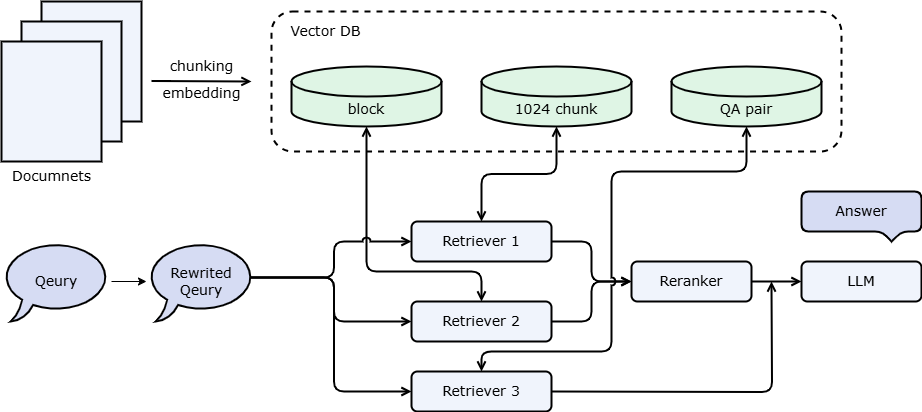
3.基于向量数据库和 vLLM 服务的 RAG 系统

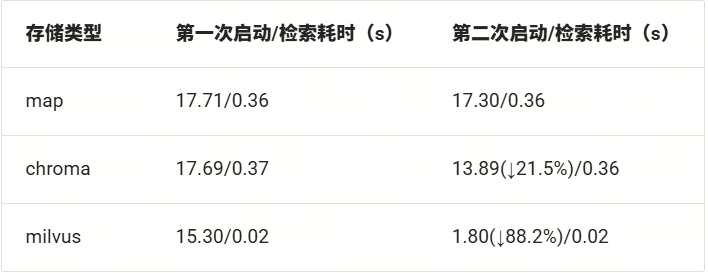
将本篇教程中的所有策略（基于向量数据库的持久化存储和高速向量搜索，vLLM启动量化推理模型）应用至进阶1 介绍的多路召回 RAG ，则得到如下代码，在同等条件下，相比于前面的版本启动时间显著减少，响应时间有一定的缩短。

 

 

我们在进阶1中提到了使用QA对的用法并推荐在学习向量数据库后进行调试，这是因为QA对提取需要耗费较长的时间和较多的token，如果每次重启系统都执行一次则会浪费大量时间和token，但如果使用了持久化存储策略，则可以每次重启系统时的等待时间，结合文档管理接口，您还可以对大模型提取的QA对进行调整和删除。

import lazyllm
from lazyllm import bind

# 使用 Milvus 存储后端
chroma_store_conf = {
  'type': 'chroma', 
  'kwargs': {
    'dir': 'qa_pair_chromadb',
   },
  'indices': {
    'smart_embedding_index': {
      'backend': 'milvus',
      'kwargs': {
        'uri': "qa_pair/test.db",
        'index_kwargs': {
          'index_type': 'HNSW',
          'metric_type': 'COSINE',
        }
      },
    },
  },
}

rewriter_prompt = "你是一个查询重写助手，负责给用户查询进行模板切换。\
          注意，你不需要进行回答，只需要对问题进行重写，使更容易进行检索\
          下面是一个简单的例子：\
          输入：RAG是啥？\
          输出：RAG的定义是什么？"
rag_prompt = 'You will play the role of an AI Q&A assistant and complete a dialogue task.'\
    ' In this task, you need to provide your answer based on the given context and question.'

# 定义嵌入模型和重排序模型
# online_embedding = lazyllm.OnlineEmbeddingModule()
embedding_model = lazyllm.TrainableModule("bge-large-zh-v1.5").start()

# 如果您要使用在线重排模型
# 目前LazyLLM仅支持 qwen和glm 在线重排模型，请指定相应的 API key。
# online_rerank = lazyllm.OnlineEmbeddingModule(type="rerank")
# 本地重排序模型
offline_rerank = lazyllm.TrainableModule('bge-reranker-large').start()

llm = lazyllm.OnlineChatModule(base_url="http://127.0.0.1:36858/v1")

qa_parser = lazyllm.LLMParser(llm, language="zh", task_type="qa")

docs = lazyllm.Document("/path/to/your/document", embed=embedding_model, store_conf=chroma_store_conf)
docs.create_node_group(name='block', transform=(lambda d: d.split('\n')))
docs.create_node_group(name='qapair', transform=qa_parser)

def retrieve_and_rerank():
    with lazyllm.pipeline() as ppl:
        with lazyllm.parallel().sum as ppl.prl:
            # CoarseChunk是LazyLLM默认提供的大小为1024的分块名
            ppl.prl.retriever1 = lazyllm.Retriever(doc=docs, group_name="CoarseChunk", index="smart_embedding_index", topk=3)
            ppl.prl.retriever2 = lazyllm.Retriever(doc=docs, group_name="block", similarity="bm25_chinese", topk=3)
        ppl.reranker = lazyllm.Reranker("ModuleReranker",
                                         model=offline_rerank,
                                         topk=3) | bind(query=ppl.input)
    return ppl

with lazyllm.pipeline() as ppl:
    # llm.share 表示复用一个大模型，如果这里设置为promptrag_prompt则会覆盖rewrite_prompt
    ppl.query_rewriter = llm.share(lazyllm.ChatPrompter(instruction=rewriter_prompt))
    with lazyllm.parallel().sum as ppl.prl:
        ppl.prl.retrieve_rerank = retrieve_and_rerank()
        ppl.prl.qa_retrieve = lazyllm.Retriever(doc=docs, group_name="qapair", index="smart_embedding_index", topk=3)      
    ppl.formatter = (
          lambda nodes, query: dict(
              context_str='\n'.join([node.get_content() for node in nodes]),
              query=query)
        ) | bind(query=ppl.input)
    ppl.llm = llm.share(lazyllm.ChatPrompter(instruction=rag_prompt, extra_keys=['context_str']))

lazyllm.WebModule(ppl, port=23491, stream=True).start().wait()

基于本节教程内容关于 LazyLLM 如何使用向量数据库实现持久化存储和高速向量检索的相关内容，可以有效减少RAG系统在重启和执行阶段的计算耗时，在某些特定节点组的角度还可以节省大量 token 费用。其次，通过灵活使用 vLLM 框架，可以得到更快的推理速度，通过使用量化模型，可以在保留相似的生成效果的条件下，压低硬件要求，节省硬件成本，也可以减少模型启动时的模型加载时间。

 

更多技术细节，欢迎移步“LazyLLM”gzh！