![]()
作者:王旭东
Databend 研发工程师
https://github.com/xudong963
IEJoin 算法可以高效的处理时序场景中的 Range(ASOF) Join。
Join conditions
Equi condition
在 下面 SQL 中
SELECT *
FROM employee JOIN department
ON employee.DepartmentID = department.DepartmentID AND
employee.ID = department.ID;
employee.DepartmentID = department.DepartmentID OR employee.ID = department.ID 都是 equi-condition,它们用 AND 连接,这条 SQL 被称为 equi-join。
Non-equi condition
condition 可以是任意的 bool 表达式,不局限于 = 和 AND。这类 condition 被称为 non-equi condition, 进一步可以细分为 Range condition 和 Other condition。
-
Range condition
- 范围比较,如
employee.DepartmentID > department.DepartmentID 就是 range condition, 这类 condition 在时序场景中非常常见。
-
Other condition
- 除了 Range condition 的其他各种奇奇怪怪的 contition, 可以被归为 Other condition, 如
OR 连接的 condition, employee.DepartmentID = department.DepartmentID OR employee.ID = department.ID。
Join condition → Join algorithm
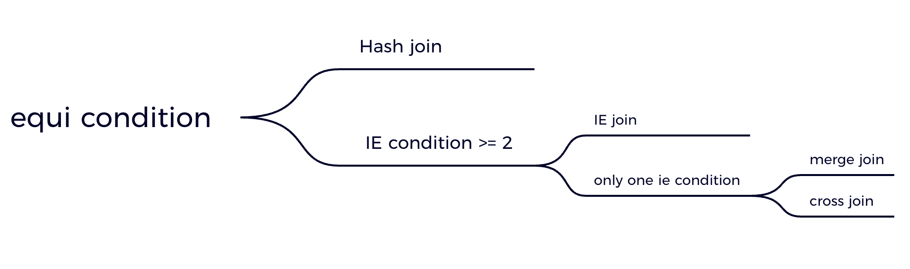
在 Databend 中,我们根据 join condition 的类别选择不同的 join 算法,使 join 能够最高效。
![]()
如果包含 equi condition,选择 hash join (即使还包含其他类型的 condition ),hash join 可以高效的利用 equi condition 过滤到一定数量的数据,剩下的数据再利用其他 condition 过滤。
如果至少两个 IE condition,选择 IEJoin,一般数据库会使用 Nested Loop Joins,非常的低效。
如果只有一个 IE condition,选择 merge join。
什么是 IEJoin,它有什么黑魔法?
IEJoin
将 join keys 涉及到的 columns 放到 sorted arrays 中,利用 permutation array 来记录一个 sorted array 中 tuples 相对于另一个 sorted array 的位置,通过 bit array 来高效的计算符合两个 IE conditions 的 tuples 的交集。
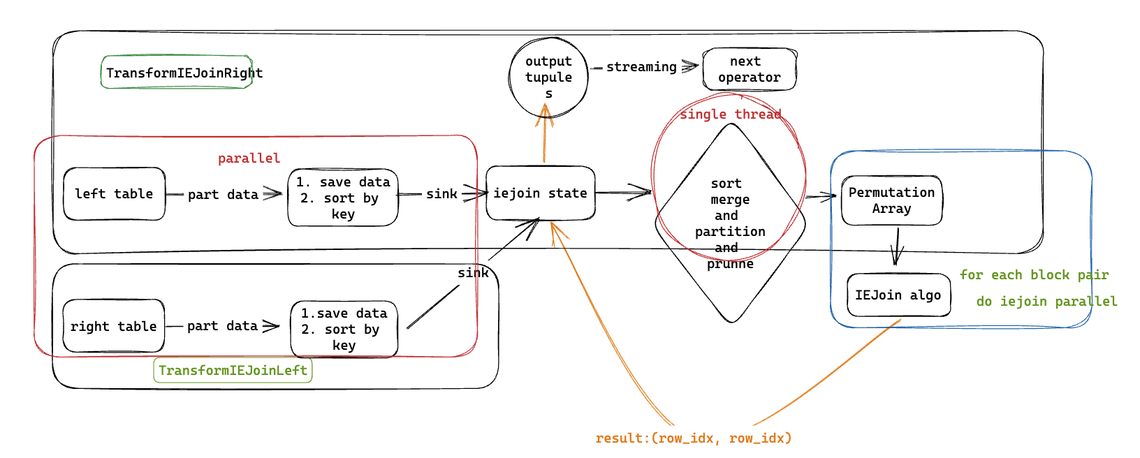
IEJoin 在整体 pipeline 架构上的设计
![]()
IEJoin 算法
mysql> select * from east;
+------+------+------+-------+
| id   | dur  | rev  | cores |
+------+------+------+-------+
|  101 |  100 |   12 |     8 |
|  102 |   90 |    5 |     4 |
|  100 |  140 |   12 |     2 |
+------+------+------+-------+

mysql> select * from west;
+------+------+------+-------+
| t_id | time | cost | cores |
+------+------+------+-------+
|  404 |  100 |    6 |     4 |
|  498 |  140 |   11 |     2 |
|  676 |   80 |   10 |     1 |
|  742 |   90 |    5 |     4 |
+------+------+------+-------+
SELECT east.id, west.id
FROM east, west
WHERE east.dur < west.time AND east.rev > west.cost
这条 SQL 在大多数数据库中都会被按照 Cross join 处理(如果数据规模很大,甚至会直接 OOM ),但是如果用 IEjoin 算法来处理,速度会得到数量级的提升 🚀
为了便于理解,首先看一条 SelfJoin 的例子
SELECT s1.t_id, s2.t_id
FROM west s1, west s2
WHERE s1.time > s2.time AND s1.cost < s2.cost
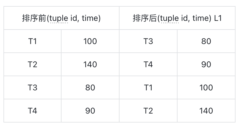
对 time 列递增排序,得到 L1
![]() 对
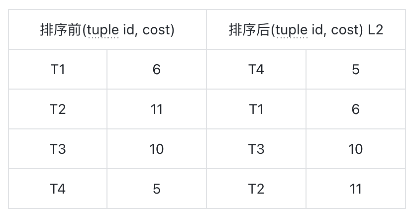
对 cost 列递增排序,得到 L2
![]()
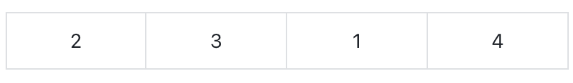
通过 L1 和 L2 可以得到 permutation array(P),P 记录了 L2 中 tuple id 在 L1 中位置
![]()
如:T4 在 L2 中的位置是1,对应到 L1 是2,所以 P 的第一个元素是 2。
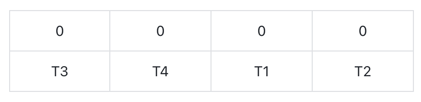
初始化 bit-array,bit-array 是基于 L1 的,初始时全部为 0。
![]()
对于 L2,后 visit 的 cost 大于先 visit 的 cost,即满足 s1.cost < s2.cost,如先访问 T4,则 bit-array 的第二个元素被设置为 1,再访问 T3 的时候,对应 bit-array 中第一个元素,它后面的第二个元素已经被设置为 1,说明 T4.cost < T3.cost,则 {T4, T3} 符合条件 s1.cost < s2.cost
对于 L1,由于 bit-array 是基于 L1 的,所以如果 bit-array 中某个位置之后的位置被设置为 1,则表明后面设为 1 的位置的 tuple id 满足 s1.time > s2.time, 如 T1 对应的位置设为 1,当访问 T3 时,T1.time > T3.time,则 {T1, T3} 符合条件 s1.time > s2.time。
bit-array 的作用就是通过标记,来找到同时满足两个 IE conditions 的 tuple pair。
算法流程
-
遍历 P, P[1] 对应 T4,T4 在 L1 中的位置是 P[1] = 2,将 bit-array 的第二个位置设为 1,由于其后位置都为 0,所以没有满足条件的结果。
-
P[2] 对应 T1,T1 在 L1 中的位置是 P[1] = 3,将 bit-array 的第三个位置设为 1,由于其后位置都为 0,所以没有满足条件的结果。
-
P[3] 对应 T3,T3 在 L1 中的位置是 P[3] = 1,将 bit-array 的第一个位置设为1,由于 bit-array 的第二/三位置都为 1,所以 {T1, T3}, {T4, T3} 满足条件。
-
P[4] 对应 T2,T2 在 L1 中的位置是 P[4] = 4,将 bit-array 的第四个位置设为 1,由于它是最后一个位置,所以没有满足条件的结果。
由 SelfJoin 拓展到不同表 join
SELECT east.id, west.id
FROM east, west
WHERE east.dur < west.time AND east.rev > west.cost
对 dur 排序得到 L1,对 rev 排序得到 L2。 L2 和 L1 比较得到 P。
对 time 排序得到 L1’,对 cost 排序得到 L2’。 L2’ 和 L1’ 比较得到 P’。
将 L1 和 L1’ 合并排序,L2 和 L2’ 合并排序,合并 P 和 P’。
最终得到了合 SelfJoin 类似的数据结构,可以应用 SelfJoin 的算法流程,但是需要处理掉重复的结果。
性能数据
M1 mac (10 core, 32G)
SQL: select count() from lineitem join orders on l_orderkey > o_orderkey and l_partkey < o_custkey;
TPCH SF 0.01
IEJoin: 0.974s, Cross join: 16.639s
TPCH SF 0.1
IEJoin: 79.085s, Cross join: OOM
Connect With Us
Databend 是一款开源、弹性、低成本,基于对象存储也可以做实时分析的新式数仓。期待您的关注,一起探索云原生数仓解决方案,打造新一代开源 Data Cloud。
 对
对